Visualizing Wavelet Packet Terminal Nodes in Wavelet Signal Analyzer
A wavelet packet decomposition of level consists of terminal nodes. By design, the Wavelet Signal Analyzer app lists and plots at most 32 terminal nodes. This example demonstrates how the app selects the nodes. The example also shows how to plot a subset of the nodes, based on the frequency range.
Import Data
Load the Kobe earthquake data set.
load kobeObtain Decimated Wavelet Packet Decomposition
Open Wavelet Signal Analyzer and import the Kobe data. By default, the app obtains the nondecimated discrete wavelet decomposition of the data. Obtain the decimated wavelet packet decomposition of the signal down to level 6 using the fk18 wavelet. The decomposition consists of nodes.
On the Analyzer tab, click Add and choose Decimated Wavelet Packet. The
kobe2scenario appears in Scenarios.On the Wavelet tab, set Wavelet to fk, Number to 18, and Level to 6.
Click Analyze to update the decomposition.
Switch back to the Analyzer tab.
Node Selection Algorithm
Recall that in the wavelet packet transform, each node (wavelet packet) corresponds to an equal-width subband filtering of the input signal. Furthermore, when you use an orthogonal wavelet to obtain the wavelet packet decomposition, you end up with a partitioning of the signal energy among the equal-width subbands. Wavelet Signal Analyzer uses the following procedure to select which nodes of a wavelet packet decomposition to list and display.
For the current frequency range,
[0,Fs/2), whereFsis the sample rate, the app determines the relative energies of the nodes in that range.The app sort the nodes by relative energy in descending order.
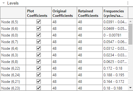
In that same order, Wavelet Signal Analyzer lists the nodes in Levels, and plots those coefficients in Decomposition Coefficients. If there are more than 32 nodes in the decomposition, the app displays the first 32 nodes.

Reproduce Order in Workspace
Reproduce the ordered list of nodes in your workspace. Click Export, and then under Decomposition Coefficients, select Generate MATLAB® Script. After a few moments, an untitled script appears in your editor. Modify the output of the dwpt function to include the center frequencies of the approximate subbands. Save the script and execute.
% Perform the decomposition using DWPT
% wpt       - Terminal nodes
% l         - Bookkeeping vector necessary for inverse DWPT
% frq       - Center frequencies of approximate subbands
% relEnergy - Energy by node as a fraction of the total energy
numberOfLevels = 6;
[wpt,l,~,frq,relEnergy] = dwpt(kobe,"fk18",Level=numberOfLevels,Boundary="periodic");

% Energy by node as a percentage of the total energy
relativeEnergyByNode = 100*cell2mat(relEnergy);
Confirm that there are 64 terminal nodes in the decomposition and the sum of the nodal energies equals 100 percent.
length(wpt)
ans =
64
sum(relativeEnergyByNode)
ans =
100.0000
Sort the nodes by relative energy in descending order. Each node corresponds to an approximate subband. List the center frequencies of the sorted subbands. Confirm that Levels lists the nodes in the same order. Keep in mind that indexing is zero-based.
[sortedRelativeEnergies,nodeIndex] = sort(relativeEnergyByNode,"descend");
reorderedCenterFrequencies = frq(nodeIndex);
nodeIndex = nodeIndex-1;
nodeList = table(nodeIndex,sortedRelativeEnergies,reorderedCenterFrequencies)nodeList=64×3 table
nodeIndex sortedRelativeEnergies reorderedCenterFrequencies
_________ ______________________ __________________________
5 28.799 0.042969
6 12.707 0.050781
0 10.72 0.0039062
7 10.001 0.058594
4 9.3465 0.035156
3 7.1272 0.027344
8 4.5254 0.066406
22 2.1989 0.17578
24 1.8151 0.19141
21 1.3272 0.16797
23 1.2751 0.18359
9 1.1619 0.074219
26 0.89599 0.20703
25 0.891 0.19922
1 0.86739 0.011719
20 0.86029 0.16016
⋮

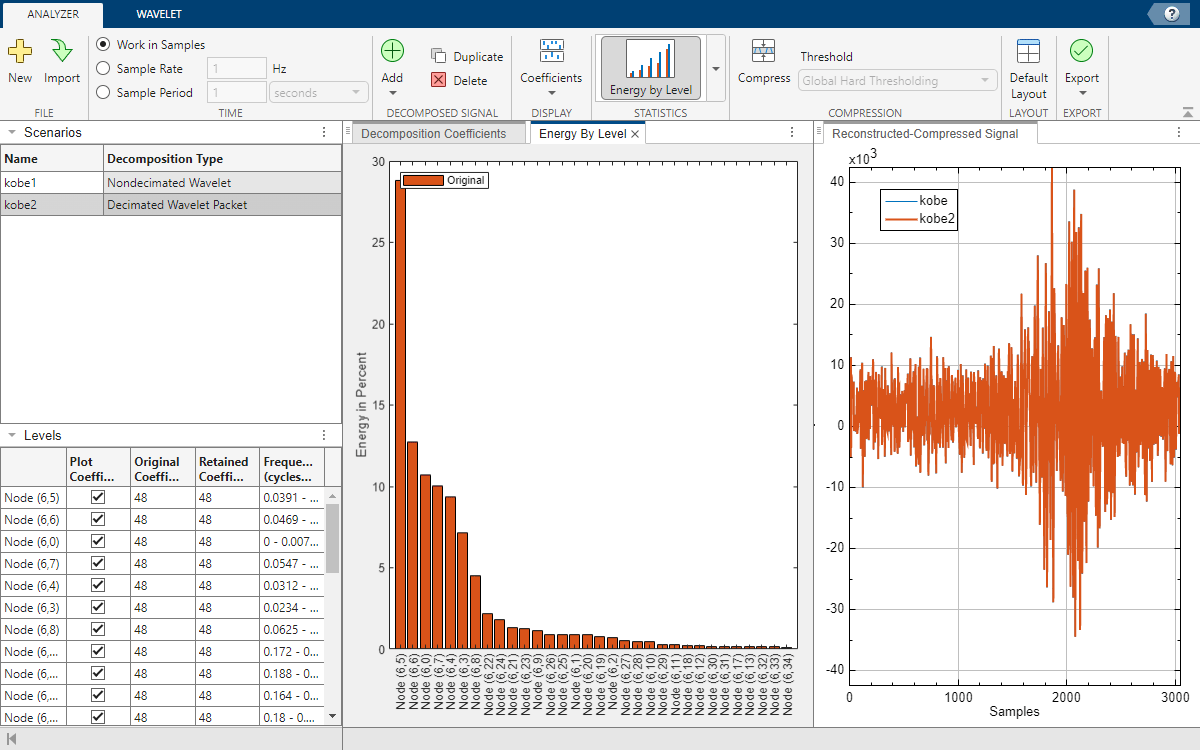
Plot the energy by level. In the Statistics section, click the arrow to open the gallery. Under For All Levels, click Energy by Level. Confirm the energies are plotted in descending order.

Display Nodes in Specific Frequency Range
By default, to determine which 32 nodes to display, Wavelet Signal Analyzer sorts the terminal nodes based on the frequency range , where is the sample rate. You can observe the terminal nodes from the following four frequency ranges:
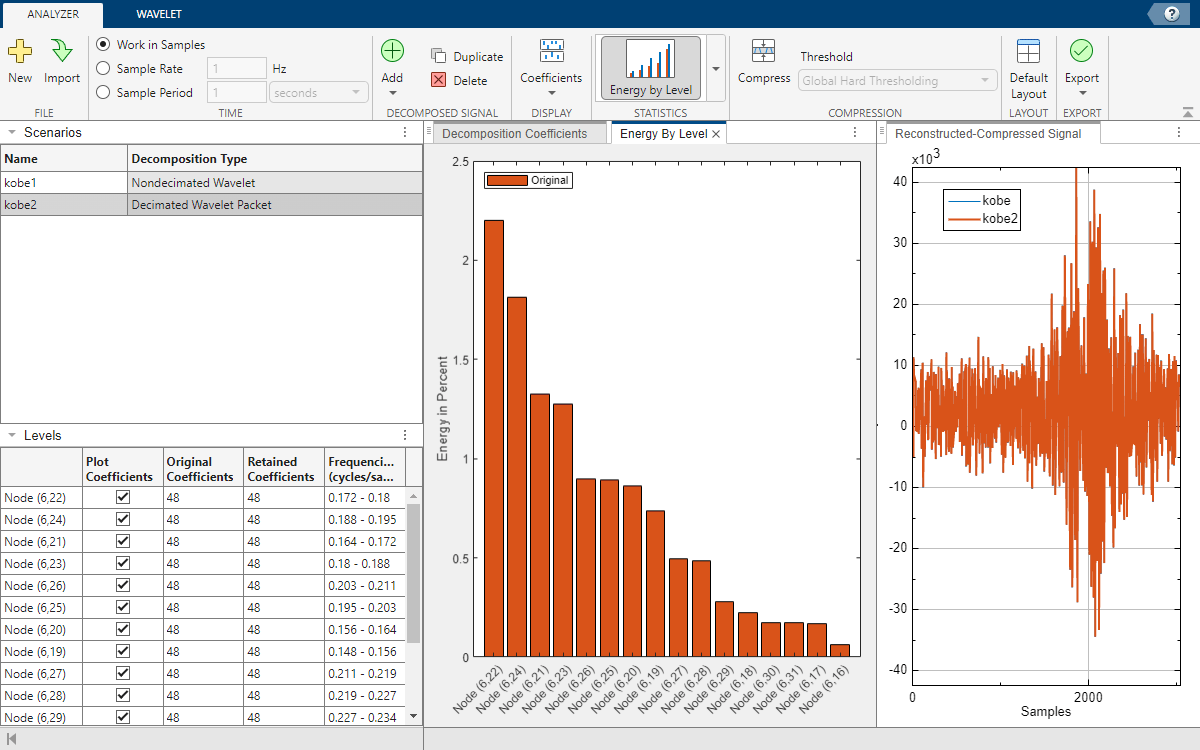
To plot the nodes with the most energy in the frequency range , click Coefficients > Terminal Nodes Selected. Under By Frequency Range, select Specify the frequency range for packet coefficients > [Fs/8,Fs/4).

The Levels table and plots update to reflect the range. The app lists and plots all 16 nodes in the range in descending order of relative energy.

Reproduce the order in your workspace.
subFreqInd = find((nodeList.reorderedCenterFrequencies >= 1/8) & ...
    (nodeList.reorderedCenterFrequencies < 1/4));
nodeList(subFreqInd,:)ans=16×3 table
nodeIndex sortedRelativeEnergies reorderedCenterFrequencies
_________ ______________________ __________________________
22 2.1989 0.17578
24 1.8151 0.19141
21 1.3272 0.16797
23 1.2751 0.18359
26 0.89599 0.20703
25 0.891 0.19922
20 0.86029 0.16016
19 0.73645 0.15234
27 0.49414 0.21484
28 0.48409 0.22266
29 0.27693 0.23047
18 0.22348 0.14453
30 0.17528 0.23828
31 0.17136 0.24609
17 0.16958 0.13672
16 0.064556 0.12891