Morse Wavelets
What Are Morse Wavelets?
Generalized Morse wavelets are a family of exactly analytic wavelets. Analytic wavelets are complex-valued wavelets whose Fourier transforms are supported only on the positive real axis. They are useful for analyzing modulated signals, which are signals with time-varying amplitude and frequency. They are also useful for analyzing localized discontinuities. The seminal paper for generalized Morse wavelets is Olhede and Walden [1]. The theory of Morse wavelets and their applications to the analysis of modulated signals is further developed in a series of papers by Lilly and Olhede [2], [3], and [4]. Efficient algorithms for the computation of Morse wavelets and their properties were developed by Lilly [5].
The Fourier transform of the generalized Morse wavelet is
where U(ω) is the unit step, is a normalizing constant, P2 is the time-bandwidth product, and characterizes the symmetry of the Morse wavelet. Much of the literature about Morse wavelets uses , which can be viewed as a decay or compactness parameter, rather than the time-bandwidth product, . The equation for the Morse wavelet in the Fourier domain parameterized by and is
For a detailed explanation of the parameterization of Morse wavelets, see [2].
By adjusting the time-bandwidth product and symmetry parameters of a Morse wavelet, you can obtain analytic wavelets with different properties and behavior. A strength of Morse wavelets is that many commonly used analytic wavelets are special cases of a generalized Morse wavelet. For example, Cauchy wavelets have = 1 and Bessel wavelets are approximated by = 8 and = 0.25. See Generalized Morse and Analytic Morlet Wavelets.
Morse Wavelet Parameters
As previously mentioned, Morse wavelets have two parameters, symmetry and
time-bandwidth product, which determine the wavelet shape and affect the behavior of
the transform. The Morse wavelet gamma parameter, , controls the symmetry of the wavelet in time through the
demodulate skewness [2]. The square root of the time-bandwidth product, P, is
proportional to the wavelet duration in time. For convenience, the Morse wavelets in
cwt and cwtfilterbank are parameterized as the time-bandwidth product and
gamma. The duration determines how many oscillations can fit into the time-domain
wavelet’s center window at its peak frequency. The peak frequency is
The (demodulate) skewness of the Morse wavelet is equal to 0 when gamma is equal
to 3. The Morse wavelets also have the minimum Heisenberg area when gamma is equal
to 3. For these reasons, cwt and cwtfilterbank use this as the default value.
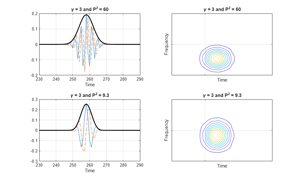
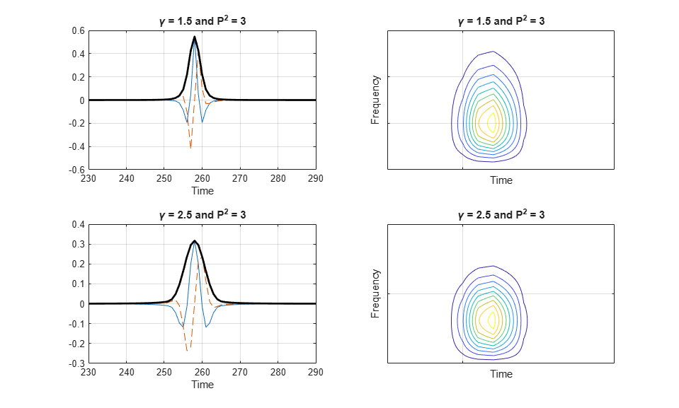
Effect of Parameter Values on Morse Wavelet Shape
These plots show how different values of symmetry and time-bandwidth affect the shape of a Morse wavelet. Longer time-bandwidths broaden the central portion of the wavelet and increase the rate of the long time decay. Increasing the symmetry broadens the wavelet envelope, but does not affect the long time decay. For symmetry values less than or equal to 3, the time decay increases as the time-bandwidth increases. For symmetry greater than or equal to 3, reducing the time-bandwidth makes the wavelet less symmetric. As both symmetry and time-bandwidth increase, the wavelet oscillates more in time and narrows in frequency. Very small time-bandwidth and large symmetry values produce undesired time-domain sidelobes and frequency-domain asymmetry.
In the time-domain plots in the left column, the red line is the real part and the blue line is the imaginary part. The contour plots in the right column show how the parameters affect the spread in time and frequency.
Relationship Between Analytic Morse Wavelet and Analytic Signal
The coefficients from a wavelet transform using an analytic wavelet on a real signal are proportional to the coefficients of the corresponding analytic signal. An analytic signal is defined as the inverse Fourier transform of
The value of the analytic signal depends on ω.
For ω > 0, the Fourier transform of an analytic signal is two times the Fourier transform of the corresponding nonanalytic signal,.
For ω = 0, the Fourier transform of an analytic signal is equal to the Fourier transform of the corresponding nonanalytic signal.
For ω < 0, the Fourier transform of an analytic signal vanishes.
Let denote the wavelet transform of a signal, f(t),
at translation u and scale s. If the analyzing
wavelet is analytic, you obtain , where fa(t) is the
analytic signal corresponding to f(t). For all wavelets used in
cwt, the amplitude of the wavelet bandpass filter at the
peak frequency for each scale is set to 2. Additionally, cwt
uses L1 normalization. For a real-valued sinusoidal input with radian frequency
ω0 and amplitude A, the wavelet
transform using an analytic wavelet yields coefficients that oscillate at the same
frequency, ω0, with an amplitude equal to . By isolating the coefficients at the scale, , a peak magnitude of 2 assures that the analyzed oscillatory
component has the correct amplitude, A.
Comparison of Analytic Wavelet Transform and Analytic Signal Coefficients
This example shows how the analytic wavelet transform of a real signal approximates the corresponding analytic signal.
This is demonstrated using a sine wave. If you obtain the wavelet transform of a sine wave using an analytic wavelet and extract the wavelet coefficients at a scale corresponding to the frequency of the sine wave, the coefficients approximate the analytic signal. For a sine wave, the analytic signal is a complex exponential of the same frequency.
Create a sinusoid with a frequency of 50 Hz. The signal is sampled at 1000 Hz for one second.
Fs = 1000;
t = 0:1/Fs:1;
x = cos(2*pi*50*t);
Obtain its continuous wavelet transform using an analytic Morse wavelet. Specify 32 voices per octave and periodic boundary extension. You must have the Signal Processing Toolbox™ to use hilbert.
[wt,f] = cwt(x,Fs,VoicesPerOctave=32,Boundary="periodic");
analytsig = hilbert(x);
Obtain the wavelet coefficients at the scale closest to the sine wave's frequency of 50 Hz.
[~,idx] = min(abs(f-50));
morsecoefx = wt(idx,:);
Compare the real and imaginary parts of the analytic signal with the wavelet coefficients at the signal frequency.
plot(t,[real(morsecoefx)' real(analytsig)'])
title("Real Parts")
ylim([-2 2])
grid on
legend("Wavelet Coefficients","Analytic Signal",Location="SouthEast")
xlabel("Time (s)")
ylabel("Amplitude")
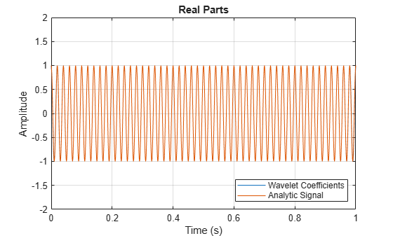
figure
plot(t,[imag(morsecoefx)' imag(analytsig)'])
title("Imaginary Parts")
ylim([-2 2])
grid on
legend("Wavelet Coefficients","Analytic Signal",Location="SouthEast")
xlabel("Time (s)")
ylabel("Amplitude")
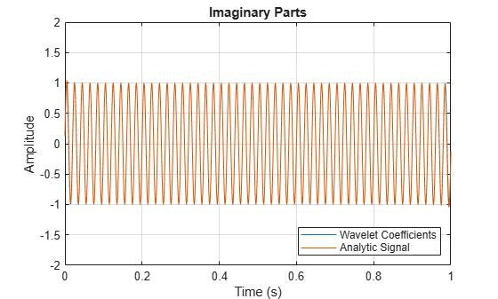
cwt uses L1 normalization and scales the wavelet bandpass filters to have a peak magnitude of 2. The factor of 1/2 in the above equation is canceled by the peak magnitude value.
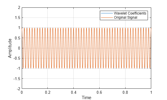
The wavelet transform represents a frequency-localized filtering of the signal. Accordingly, the CWT coefficients are less sensitive to noise than are the Hilbert transform coefficients.
Add highpass noise to the signal and reexamine the wavelet coefficients and the analytic signal.
y = x + filter(1,[1 0.9],0.1*randn(size(x)));
analytsig = hilbert(y);
[wt,f] = cwt(y,1000,VoicesPerOctave=32,Boundary="periodic");
morsecoefy = wt(idx,:);

plot(t,[real(analytsig)' x'])
legend("Analytic Signal","Original Signal")
grid on
xlabel("Time")
ylabel("Amplitude")
ylim([-2 2])
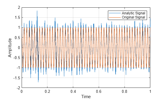
figure
plot(t,[real(morsecoefy)' x'])
legend("Wavelet Coefficients","Original Signal")
grid on
xlabel("Time")
ylabel("Amplitude")
ylim([-2 2])
Recommended Morse Wavelet Settings for the CWT
For the best results when using the CWT, use a symmetry, , of 3, which is the default for cwt and
cwtfilterbank. With gamma fixed, increasing the time-bandwidth
product narrows the wavelet filter in frequency while increasing the width
of the central portion of the filter in time. It also increases the number of
oscillations of the wavelet under the central portion of the filter.
References
[1] Olhede, S. C., and A. T. Walden. “Generalized morse wavelets.” IEEE Transactions on Signal Processing, Vol. 50, No. 11, 2002, pp. 2661-2670.
[2] Lilly, J. M., and S. C. Olhede. “Higher-order properties of analytic wavelets.” IEEE Transactions on Signal Processing, Vol. 57, No. 1, 2009, pp. 146-160.
[3] Lilly, J. M., and S. C. Olhede. “On the analytic wavelet transform.” IEEE Transactions on Information Theory, Vol. 56, No. 8, 2010, pp. 4135–4156.
[4] Lilly, J. M., and S. C. Olhede. “Generalized Morse wavelets as a superfamily of analytic wavelets.” IEEE Transactions on Signal Processing Vol. 60, No. 11, 2012, pp. 6036-6041.
[5] Lilly, J. M. jLab: A data analysis package for MATLAB®, version 1.6.2., 2016. http://www.jmlilly.net/jmlsoft.html.
[6] Lilly, J. M. “Element analysis: a wavelet-based method for analysing time-localized events in noisy time series.” Proceedings of the Royal Society A. Volume 473: 20160776, 2017, pp. 1–28. dx.doi.org/10.1098/rspa.2016.0776.