HDL Implementation of IQ Imbalance Estimation and Compensation
This example shows how to implement IQ imbalance estimation and compensation on QAM/PSK modulated signals using Simulink®. The Simulink blocks used in this example are optimized for HDL code generation and hardware implementation.
The I/Q imbalance is a common problem in radio frequency (RF) front-ends using analog quadrature down-mixing. In this process, the incoming RF signal is split into in-phase (I) and quadrature-phase (Q) arms. When I/Q imbalance arises, it causes a mismatch between these two arms, leading to a range of problems that can significantly affect the demodulation performance of the receiver. One of the key effects of I/Q imbalance is the distortion it causes in both the amplitude and phase of the signals in the in-phase and quadrature-phase arms. The imbalance leads to deviations from the ideal amplitude and phase relationships between these components. As a result, the demodulation process becomes less accurate, which lowers the signal quality and system quality.
Model Architecture
Direct conversion receivers, in particular, introduce IQ imbalance. You can compensate the imbalance between in-phase and quadrature-phase components of the RF receiver signal effectively without investing on the analog front-end RF hardware. The IQ imbalance compensator in this example is developed based on the circularity-based blind compensation algorithm. For more information about this algorithm, see the Algorithms section in the comm.IQImbalanceCompensator System object™ documentation.
This figure shows the high-level overview of the Imbalance Estimation and Correction model in this example. The IQImbEstAndComp subsystem accepts IQ effected QAM/PSK signals and compensates their IQ imbalance using a compensating coefficient.
modelName = 'HDLIQImbalanceEstimatorAndCompensator';
open_system(modelName);
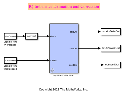
You can specify the compensating coefficient through the input port coeffIn or you can generate it from the input signal.
open_system([modelName '/IQImbEstAndComp'],'force')
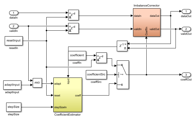
If you set Source for compensator coefficient parameter to Input port, the ImbalanceCorrector subsystem accepts compensator coefficient from the input port coeffIn.
If you set Source for compensator coefficient parameter to Estimate from input signal, the CoefficientEstimator subsystem determines the coefficient from the input signal using blind adaptive estimation algorithm. Later, the ImbalanceCorrector subsystem uses this coefficient.
Generate Input
Generate input data by using the QPSK modulation. Introduce additive white Gaussian noise (AWGN) to simulate realistic channel conditions. Further, apply IQ imbalance to the signal. This involves adjusting both the amplitude and phase imbalance parameters to test the robustness of the receiver against common RF impairments.
M = 4;
spf = 1e6*log2(M);
data = randi([0 1],spf,1);
txSig = qammod(data,M,'InputType', 'bit','UnitAveragePower', true);

% Add AWGN to the QPSK modulated signal
snr = 15;
awgnSig = awgn(txSig,snr);

% Apply IQ imbalance
ampImb = 20;  % dB
phImb = 10;  % degrees
rxSig = iqimbal(awgnSig,ampImb,phImb);

% Generate inputs to the Simulink model
simDataIn = rxSig;
simValidIn = true(size(simDataIn));
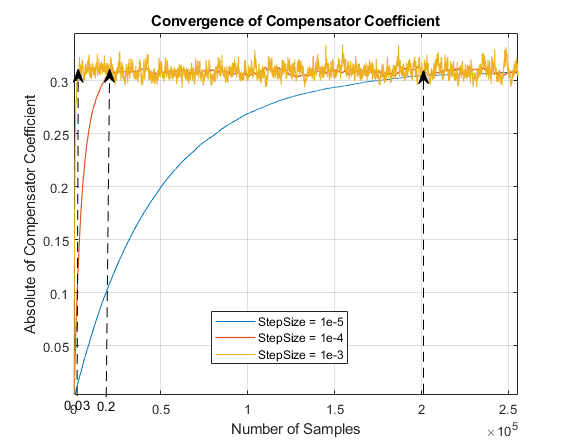
The CoefficientEstimator subsystem uses Initial compensator coefficient and Adaptation step size from the block mask to determine the compensator coefficient.
By default, the initial coefficient is specified as '0 + 0i'. You can modify the Initial compensator coefficient considering the system characteristics, signal properties or any previously measured data. A well-selected initial coefficient improves the coefficient convergence.
The step-size, also known as the adaptation or update step, determines the extent of adjustment applied to the compensation coefficients during each iteration of the estimation algorithm. It plays a crucial role in achieving a balance between the convergence speed and stability. Optimal selection of the step-size enables the IQ imbalance estimation algorithm to converge efficiently and accurately determine the compensation coefficients, resulting in effective correction of the imbalance and improved demodulation performance. The figure shows the convergence of the coefficient for different step sizes.
Run Model
Simulate the model with the above generated inputs simDataIn and simValidIn. The model estimates and compensates the IQ imbalance in the input signal. After compensation, the model outputs the compensated output and the compensator coefficient.
out = sim(modelName);
Verify Compensated Output
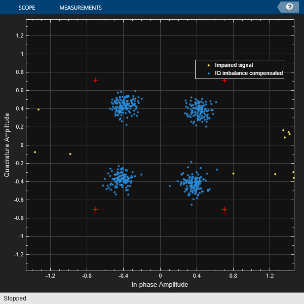
Collect the compensated data output and compensator coefficient for verification. To view the effects of IQ imbalance, the example displays the constellation. Calculate the error vector magnitude (EVM) to estimate the improvement in the signal quality after compensation.
compSig = double(out.simDataOut(out.simValidOut));
coeffOut = double(out.coeffOut(out.simValidOut));

% Display Constellation
cdscope = comm.ConstellationDiagram( ...
    'Name','Effect of IQ Imbalance', ...
    'ShowReferenceConstellation',1, ...
    'NumInputPorts',2, ...
    'ShowLegend',true, ...
    'EnableMeasurements',0, ...
    'ChannelNames',["Impaired signal","IQ imbalance compensated"]);

cdscope(rxSig(end-500:end),compSig(end-500:end))
release(cdscope)

% Display estimated amplitude and phase
[a,p]=iqcoef2imbal(coeffOut(end));
fprintf('\nAmplitude Imbalance in dB = %d \n',a);
fprintf('Phase Imbalance in degrees = %d \n',p);

% Calculate EVM
evm = comm.EVM;
rmsEVMComp = evm(txSig,compSig);
release(evm)
rmsEVMUnComp = evm(txSig,rxSig);
fprintf('\nEVM of impaired signal = %d%%  \n',ceil(rmsEVMUnComp));
fprintf('EVM of IQ Compensated signal = %d%% \n',ceil(rmsEVMComp));
Amplitude Imbalance in dB = 2.003813e+01
Phase Imbalance in degrees = 1.010235e+01

EVM of impaired signal = 166%
EVM of IQ Compensated signal = 45%
Generate HDL Code
To generate HDL code for this example, you must have an HDL Coder™ license. Use the makehdl and makehdltb commands to generate HDL code and HDL test bench for the IQImbEstAndComp subsystem.
You can synthesize the generated HDL code and target on the AMD® Zynq®-7000 ZC706 evaluation board and achieve a synthesis frequency of 260 MHz. The table shows the post place and route resource utilization results.
F = table(...
    categorical({'Slice LUT'; 'Slice Registers';'DSP'}), ...
    categorical({'950'; '1421'; '13'}), ...
    categorical({'218600'; '437200'; '900'}), ...
    categorical({'0.43'; '0.33'; '1.44'}), ...
    'VariableNames', ...
    {'Resources','Utilized','Available','Utilization (%)'});
disp(F);
       Resources       Utilized    Available    Utilization (%)
    _______________    ________    _________    _______________

    Slice LUT            950        218600           0.43
    Slice Registers      1421       437200           0.33
    DSP                  13         900              1.44
References
Anttila, L., M. Valkama, and M. Renfors. "Blind Compensation of Frequency-Selective I/Q Imbalances in Quadrature Radio Receivers: Circularity-Based Approach", Proc. IEEE ICASSP, pp.III–245–248, 2007.
Kiayani, A., L. Anttila, Y. Zou, and M. Valkama, "Advanced Receiver Design for Mitigating Multiple RF Impairments in OFDM Systems: Algorithms and RF Measurements", Journal of Electrical and Computer Engineering, Vol. 2012.
See Also
comm.IQImbalanceCompensator | iqcoef2imbal | iqimbal2coef