2D Convolution Theorem
( All the details are in my blog post here: http://heraqi.blogspot.com.eg/2016/12/verifying-convolution-theorem-on-2d.html )
In our verification experiment, we will apply it to three different images with different level of details: high, medium, and low details. The reason will be clear at the end of this post.
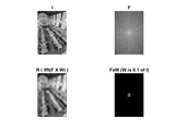
Firstly, let's create a black image W of the same size of I with a small white rectangle in the middle.
For the image I, firstly, we will get the result of multiplying the frequency domain of I by W:
1- Apply Fourier transform on I, let the result be F
2- Calculate the point-wise multiplication of F and W, let the result be F×W
3- Get the inverse Fourier transform of F×W, let this result be R1
Now, let's do the inverse process, for the same image I, we will get the result of the convolution of the spacial domain of I and the inverse Fourier transform of W.
1- Apply inverse Fourier transform on W, let the result be M
2- Calculate the convolution of I and M, let the result be R2
As described in the blog post, the convolution theorem establish that the two processes described above to get R1 and R2 are equivalent; so R1 and R2 should be the same images at the end. If we see that, we verify the convolution theorem on 2D images.
Cite As
Hesham Eraqi (2026). 2D Convolution Theorem (https://www.mathworks.com/matlabcentral/fileexchange/60897-2d-convolution-theorem), MATLAB Central File Exchange. Retrieved .
MATLAB Release Compatibility
Platform Compatibility
Windows macOS LinuxCategories
- Image Processing and Computer Vision > Image Processing Toolbox > Image Filtering and Enhancement > Image Filtering >
Tags
Discover Live Editor
Create scripts with code, output, and formatted text in a single executable document.
| Version | Published | Release Notes | |
|---|---|---|---|
| 1.0.0.0 |
More tags
|

