Main Content

maxflow

Maximum flow in graph

Description

example

mf = maxflow(G,s,t) returns the maximum flow between nodes s and t. If graph G is unweighted (that is, G.Edges does not contain the variable Weight), then maxflow treats all graph edges as having a weight equal to 1.

example

mf = maxflow(G,s,t,algorithm) specifies the maximum flow algorithm to use. This syntax is only available if G is a directed graph.

example

[mf,GF] = maxflow(___) also returns a directed graph object, GF, using any of the input arguments in previous syntaxes. GF is formed using only the edges in G that have nonzero flow values.

example

[mf,GF,cs,ct] = maxflow(___) additionally returns the source and target node IDs, cs and ct, representing the minimum cut associated with the maximum flow.

Examples

collapse all

Create and plot a weighted graph. The weighted edges represent flow capacities.

s = [1 1 2 2 3 4 4 4 5 5];
t = [2 3 3 4 5 3 5 6 4 6];
weights = [0.77 0.44 0.67 0.75 0.89 0.90 2 0.76 1 1];
G = digraph(s,t,weights);
plot(G,'EdgeLabel',G.Edges.Weight,'Layout','layered');

Figure contains an axes object. The axes object contains an object of type graphplot.

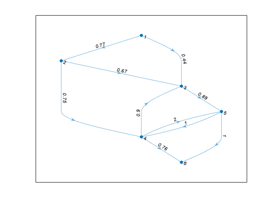
Determine the maximum flow from node 1 to node 6.

mf = maxflow(G,1,6)
mf = 1.2100

Create and plot a graph. The weighted edges represent flow capacities.

s = [1 1 2 2 3 3 4];
t = [2 3 3 4 4 5 5];
weights = [10 6 15 5 10 3 8];
G = digraph(s,t,weights);
H = plot(G,'EdgeLabel',G.Edges.Weight);

Figure contains an axes object. The axes object contains an object of type graphplot.

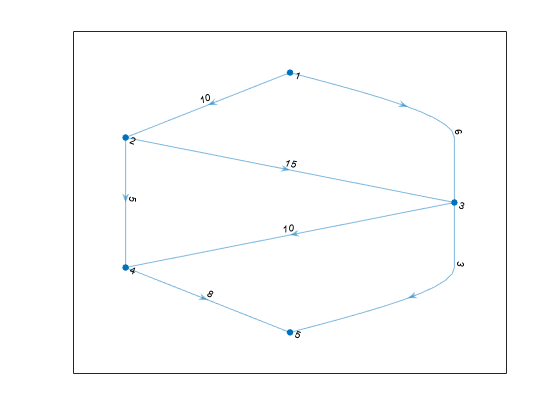
Find the maximum flow value between node 1 and node 5. Specify 'augmentpath' to use the Ford-Fulkerson algorithm, and use two outputs to return a graph of the nonzero flows.

[mf,GF] = maxflow(G,1,5,'augmentpath')
mf = 11
GF = 
  digraph with properties:

    Edges: [6x2 table]
    Nodes: [5x0 table]

Highlight and label the graph of nonzero flows.

H.EdgeLabel = {};
highlight(H,GF,'EdgeColor','r','LineWidth',2);
st = GF.Edges.EndNodes;
labeledge(H,st(:,1),st(:,2),GF.Edges.Weight);

Figure contains an axes object. The axes object contains an object of type graphplot.

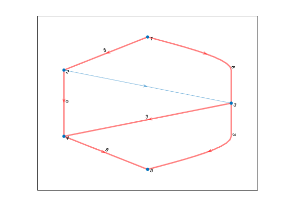
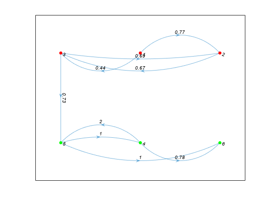
Create and plot a weighted graph. The edge weights represent flow capacities.

s = [1 1 2 3 3 4 4 5 5];
t = [2 3 3 2 5 5 6 4 6];
weights = [0.77 0.44 0.67 0.69 0.73 2 0.78 1 1];
G = digraph(s,t,weights);
plot(G,'EdgeLabel',G.Edges.Weight,'Layout','layered')

Figure contains an axes object. The axes object contains an object of type graphplot.

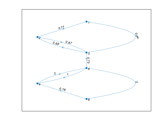
Find the maximum flow and minimum cut of the graph.

[mf,~,cs,ct] = maxflow(G,1,6)
mf = 0.7300
cs = 3×1

     1
     2
     3

ct = 3×1

     4
     5
     6

Plot the minimum cut, using the cs nodes as sources and the ct nodes as sinks. Highlight the cs nodes as red and the ct nodes as green. Note that the weight of the edge that connects these two sets of nodes is equal to the maximum flow.

H = plot(G,'Layout','layered','Sources',cs,'Sinks',ct, ...
    'EdgeLabel',G.Edges.Weight);
highlight(H,cs,'NodeColor','red')
highlight(H,ct,'NodeColor','green')

Figure contains an axes object. The axes object contains an object of type graphplot.

Input Arguments

collapse all

Input graph, specified as either a graph or digraph object. Use graph to create an undirected graph or digraph to create a directed graph.

Example: G = graph(1,2)

Example: G = digraph([1 2],[2 3])

Node pair, specified as separate arguments of node indices or node names to indicate the source node and target node. This table shows the different ways to refer to nodes either by their node indices or by their node names.

ValueExample
Scalar node index1
Character vector node name'A'
String scalar node name"A"

Example: mf = maxflow(G,'A','B')

Example: mf = maxflow(G,1,10)

Data Types: double | char | string

Maximum flow algorithm, specified as one of the entries in the table.

Note

You can only specify nondefault algorithm options with a directed graph.

OptionDescription
'searchtrees' (default)

Uses the Boykov-Kolmogorov algorithm. Computes the maximum flow by constructing two search trees associated with nodes s and t.

'augmentpath'

Uses the Ford-Fulkerson algorithm. Computes the maximum flow iteratively by finding an augmenting path in a residual directed graph.

The directed graph cannot have any parallel edges of opposite direction between the same two nodes, unless the weight of one of those edges is zero. So if the graph contains edge [i j], then it can contain the reverse edge [j i] only if the weight of [i j] is zero and/or the weight of [j i] is zero.

'pushrelabel'

Computes the maximum flow by pushing a node's excess flow to its neighbors and then relabeling the node.

The directed graph cannot have any parallel edges of opposite direction between the same two nodes, unless the weight of one of those edges is zero. So if the graph contains edge [i j], then it can contain the reverse edge [j i] only if the weight of [i j] is zero and/or the weight of [j i] is zero.

Example: mf = maxflow(G,'A','D','augmentpath')

Output Arguments

collapse all

Maximum flow, returned as a scalar.

Directed graph of flows, returned as a digraph object. GF contains the same nodes as G, but only contains those edges of G that have a nonzero flow. For multigraphs with multiple edges between the same two nodes, GF contains a single edge reflecting the flow through the multiple edges.

Minimum cut source node IDs, returned as node indices or node names.

  • If s and t specify numeric node indices, then cs and ct also contain node indices.

  • If s and t specify node names, then cs and ct also contain node names.

Minimum cut target node IDs, returned as node indices or node names.

  • If s and t specify numeric node indices, then cs and ct also contain node indices.

  • If s and t specify node names, then cs and ct also contain node names.

More About

collapse all

Maximum Flow

In the context of maximum flow, the edges in a graph are considered to have a capacity as represented by the edge weight. The capacity of an edge is the amount of flow that can pass through that edge. Therefore, the maximum flow between two nodes in a graph maximizes the amount of flow passing from the source node, s, to the target node, t, based on the capacities of the connecting edges.

Minimum Cut

A minimum cut partitions the directed graph nodes into two sets, cs and ct, such that the sum of the weights of all edges connecting cs and ct (weight of the cut) is minimized. The weight of the minimum cut is equal to the maximum flow value, mf.

The entries in cs and ct indicate the nodes of G associated with nodes s and t, respectively. cs and ct satisfy numel(cs) + numel(ct) = numnodes(G).

Extended Capabilities

Thread-Based Environment
Run code in the background using MATLAB® backgroundPool or accelerate code with Parallel Computing Toolbox™ ThreadPool.

Version History

Introduced in R2015b

See Also

|