graph
Graph with undirected edges
Description
graph objects represent undirected graphs, which have
direction-less edges connecting the nodes. After you create a graph object, you can
learn more about the graph by using object functions to perform queries against the
object. For example, you can add or remove nodes or edges, determine the shortest path
between two nodes, or locate a specific node or edge.
G = graph([1 1], [2 3]);
e = G.Edges
G = addedge(G,2,3)
G = addnode(G,4)
plot(G)
Creation
Syntax
Description
G = graphG, which has no nodes or
edges.
G = graph(A)A.
For logical adjacency matrices, the graph has no edge weights.
For nonlogical adjacency matrices, the graph has edge weights. The location of each nonzero entry in
Aspecifies an edge for the graph, and the weight of the edge is equal to the value of the entry. For example, ifA(2,1) = 10, thenGcontains an edge between node 2 and node 1 with a weight of 10.
G = graph(s,t)(s,t) in node pairs.
s and t can specify node indices
or node names. graph sorts the edges in
G first by source node, and then by target node. If
you have edge properties that are in the same order as s
and t, use the syntax G =
graph(s,t,EdgeTable) to pass in the edge properties so that
they are sorted in the same manner in the resulting graph.
G = graph(s,t,___,'omitselfloops')k
that satisfies s(k) == t(k) is ignored. You can use any
of the input argument combinations in previous syntaxes.
G = graph(EdgeTable)EdgeTable to define the graph. With this
syntax, the first variable in EdgeTable must be named
EndNodes, and it must be a two-column array defining
the edge list of the graph.
G = graph(EdgeTable,___,'omitselfloops')k that
satisfies EdgeTable.EndNodes(k,1) ==
EdgeTable.EndNodes(k,2) is ignored. You must specify
EdgeTable and optionally can specify
NodeTable.
Input Arguments
Properties
Object Functions
Examples
Create and Modify Graph Object
Create a graph object with three nodes and two edges. One edge is between node 1 and node 2, and the other edge is between node 1 and node 3.
G = graph([1 1],[2 3])
G =
  graph with properties:

    Edges: [2x1 table]
    Nodes: [3x0 table]
View the edge table of the graph.
G.Edges
ans=2×1 table
    EndNodes
    ________

     1    2
     1    3
Add node names to the graph, and then view the new node and edge tables. The end nodes of each edge are now expressed using their node names.
G.Nodes.Name = {'A' 'B' 'C'}';
G.Nodesans=3×1 table
Name
_____
{'A'}
{'B'}
{'C'}
G.Edges
ans=2×1 table
       EndNodes
    ______________

    {'A'}    {'B'}
    {'A'}    {'C'}
You can add or modify extra variables in the Nodes and Edges tables to describe attributes of the graph nodes or edges. However, you cannot directly change the number of nodes or edges in the graph by modifying these tables. Instead, use the addedge, rmedge, addnode, or rmnode functions to modify the number of nodes or edges in a graph.
For example, add an edge to the graph between nodes 2 and 3 and view the new edge list.
G = addedge(G,2,3)
G =
  graph with properties:

    Edges: [3x1 table]
    Nodes: [3x1 table]
G.Edges
ans=3×1 table
       EndNodes
    ______________

    {'A'}    {'B'}
    {'A'}    {'C'}
    {'B'}    {'C'}
Adjacency Matrix Graph Construction
Create a symmetric adjacency matrix, A, that creates a complete graph of order 4. Use a logical adjacency matrix to create a graph without weights.
A = ones(4) - diag([1 1 1 1])
A = 4×4

     0     1     1     1
     1     0     1     1
     1     1     0     1
     1     1     1     0
G = graph(A~=0)
G =
  graph with properties:

    Edges: [6x1 table]
    Nodes: [4x0 table]
View the edge list of the graph.
G.Edges
ans=6×1 table
    EndNodes
    ________

     1    2
     1    3
     1    4
     2    3
     2    4
     3    4
Adjacency Matrix Construction with Node Names
Create an upper triangular adjacency matrix.
A = triu(magic(4))
A = 4×4

    16     2     3    13
     0    11    10     8
     0     0     6    12
     0     0     0     1
Create a graph with named nodes using the adjacency matrix. Specify 'omitselfloops' to ignore the entries on the diagonal of A, and specify type as 'upper' to indicate that A is upper-triangular.
names = {'alpha' 'beta' 'gamma' 'delta'};
G = graph(A,names,'upper','omitselfloops')
G =
graph with properties:
Edges: [6x2 table]
Nodes: [4x1 table]
View the edge and node information.
G.Edges
ans=6×2 table
           EndNodes           Weight
    ______________________    ______

    {'alpha'}    {'beta' }       2
    {'alpha'}    {'gamma'}       3
    {'alpha'}    {'delta'}      13
    {'beta' }    {'gamma'}      10
    {'beta' }    {'delta'}       8
    {'gamma'}    {'delta'}      12
G.Nodes
ans=4×1 table
      Name
    _________

    {'alpha'}
    {'beta' }
    {'gamma'}
    {'delta'}
Edge List Graph Construction
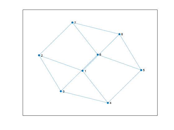
Create and plot a cube graph using a list of the end nodes of each edge.
s = [1 1 1 2 2 3 3 4 5 5 6 7];
t = [2 4 8 3 7 4 6 5 6 8 7 8];
G = graph(s,t)
G =
  graph with properties:

    Edges: [12x1 table]
    Nodes: [8x0 table]
plot(G)
Edge List Graph Construction with Node Names and Edge Weights
Create and plot a cube graph using a list of the end nodes of each edge. Specify node names and edge weights as separate inputs.
s = [1 1 1 2 2 3 3 4 5 5 6 7];
t = [2 4 8 3 7 4 6 5 6 8 7 8];
weights = [10 10 1 10 1 10 1 1 12 12 12 12];
names = {'A' 'B' 'C' 'D' 'E' 'F' 'G' 'H'};
G = graph(s,t,weights,names)
G =
graph with properties:
Edges: [12x2 table]
Nodes: [8x1 table]
plot(G,'EdgeLabel',G.Edges.Weight)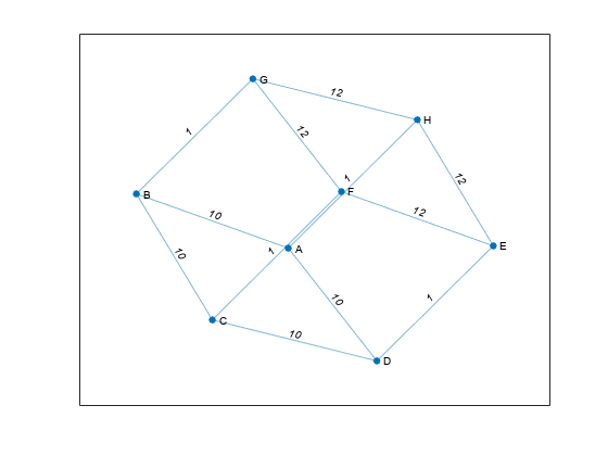
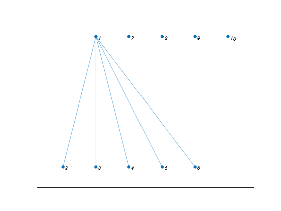
Edge List Construction with Extra Nodes
Create a weighted graph using a list of the end nodes of each edge. Specify that the graph should contain a total of 10 nodes.
s = [1 1 1 1 1];
t = [2 3 4 5 6];
weights = [5 5 5 6 9];
G = graph(s,t,weights,10)
G =
  graph with properties:

    Edges: [5x2 table]
    Nodes: [10x0 table]
Plot the graph. The extra nodes are disconnected from the primary connected component.
plot(G)
Add Nodes and Edges to Empty Graph
Create an empty graph object, G.
G = graph;
Add three nodes and three edges to the graph. The corresponding entries in s and t define the end nodes of the graph edges. addedge automatically adds the appropriate nodes to the graph if they are not already present.
s = [1 2 1];
t = [2 3 3];
G = addedge(G,s,t)
G =
  graph with properties:

    Edges: [3x1 table]
    Nodes: [3x0 table]
View the edge list. Each row describes an edge in the graph.
G.Edges
ans=3×1 table
    EndNodes
    ________

     1    2
     1    3
     2    3
For the best performance, construct graphs all at once using a single call to graph. Adding nodes or edges in a loop can be slow for large graphs.
Graph Construction with Tables
Create an edge table that contains the variables EndNodes, Weight, and Code. Then create a node table that contains the variables Name and Country. The variables in each table specify properties of the graph nodes and edges.
s = [1 1 1 2 3];
t = [2 3 4 3 4];
weights = [6 6.5 7 11.5 17]';
code = {'1/44' '1/49' '1/33' '44/49' '49/33'}';
EdgeTable = table([s' t'],weights,code, ...
'VariableNames',{'EndNodes' 'Weight' 'Code'})EdgeTable=5×3 table
EndNodes Weight Code
________ ______ _________
1 2 6 {'1/44' }
1 3 6.5 {'1/49' }
1 4 7 {'1/33' }
2 3 11.5 {'44/49'}
3 4 17 {'49/33'}
names = {'USA' 'GBR' 'DEU' 'FRA'}';
country_code = {'1' '44' '49' '33'}';
NodeTable = table(names,country_code,'VariableNames',{'Name' 'Country'})NodeTable=4×2 table
Name Country
_______ _______
{'USA'} {'1' }
{'GBR'} {'44'}
{'DEU'} {'49'}
{'FRA'} {'33'}
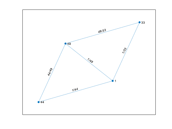
Create a graph using the node and edge tables. Plot the graph using the country codes as node and edge labels.
G = graph(EdgeTable,NodeTable);
plot(G,'NodeLabel',G.Nodes.Country,'EdgeLabel',G.Edges.Code)
Extended Capabilities
Version History
Introduced in R2015bYou can also select a web site from the following list:
Americas
- América Latina (Español)
- Canada (English)
- United States (English)
Europe
- Belgium (English)
- Denmark (English)
- Deutschland (Deutsch)
- España (Español)
- Finland (English)
- France (Français)
- Ireland (English)
- Italia (Italiano)
- Luxembourg (English)
- Netherlands (English)
- Norway (English)
- Österreich (Deutsch)
- Portugal (English)
- Sweden (English)
- Switzerland
- United Kingdom (English)