pmtm
Multitaper power spectral density estimate
Syntax
Description
pxx = pmtm(x)pxx, of the
input signal x using Discrete Prolate Spheroidal (Slepian) Sequences as tapers.
pxx = pmtm(x,m,Tapers="sine")
[___] = pmtm(___,
returns the multitaper PSD estimate over the frequency range specified by
freqRange)freqRange.
[___] = pmtm(___,DropLastTaper=
specifies whether tf)pmtm drops the last Slepian taper when computing the
multitaper PSD estimate.
[___] = pmtm(___,
combines the individual tapered PSD estimates using the method specified in
method)method. This syntax applies only to Slepian tapers.
[___] = pmtm(
uses the cell array x,dpssParams,___)dpssParams to pass input arguments to
dpss. This syntax applies only to Slepian tapers.
pmtm(___) with no output arguments plots the multitaper
PSD estimate in the current figure window.
Examples
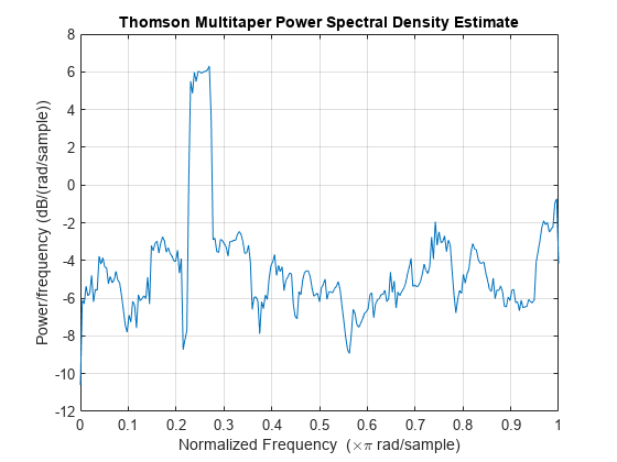
Obtain the multitaper PSD estimate of an input signal consisting of a discrete-time sinusoid with an angular frequency of rad/sample with additive N(0,1) white noise.
Create a sine wave with an angular frequency of rad/sample with additive N(0,1) white noise. The signal is 320 samples in length. Obtain the multitaper PSD estimate using the default time-halfbandwidth product of 4 and DFT length. The default number of DFT points is 512. Because the signal is real-valued, the PSD estimate is one-sided and there are 512/2+1 points in the PSD estimate.
rng("default")
n = 0:319;
x = cos(pi/4*n) + randn(size(n));
pxx = pmtm(x);
Plot the multitaper PSD estimate.
pmtm(x)
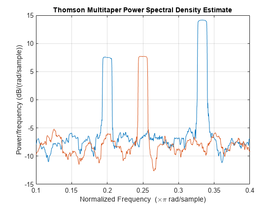
Generate 2048 samples of a two-channel signal embedded in additive N(0,1) white Gaussian noise.
The first channel consists of two sinusoids with normalized frequencies of π/3 and π/5 rad/sample. The first sinusoid has twice the amplitude of the second.
The second channel has a normalized frequency of π/4 rad/sample.
Use the multitaper method to estimate the PSD of the signal over a 1024-sample interval from 0.1π rad/sample to 0.4π rad/sample. Use 13 sine tapers weighted equally.
rng("default")
n = (0:2047)';
x = [sin(pi./[3 5].*n)*[2 1]' sin(pi/4*n)] + randn(length(n),2);
w = linspace(0.1,0.4,1024);
ntp = 13;

pmtm(x,ntp,w*pi,Tapers="sine")
Repeat the computation, but now weight the 13 tapers in linear descending order. You can place the Tapers="sine" name-value argument anywhere after x in the function call.
pmtm(x,(ntp:-1:1)/sum(1:ntp),w*pi,Tapers="sine")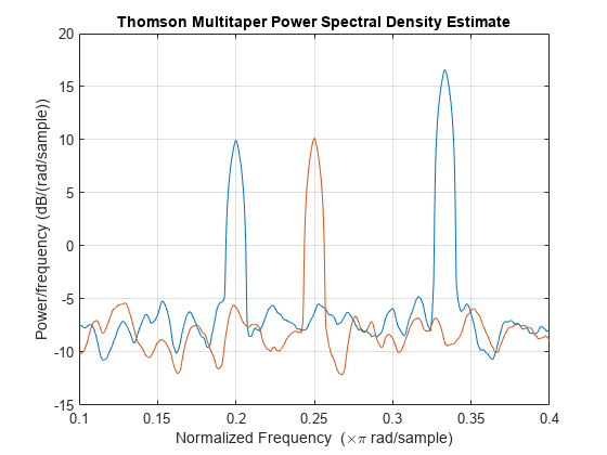
Repeat the computation, but now use 13 Slepian tapers and specify a time-halfbandwidth product of 7.5.
nw = 7.5;

pmtm(x,{nw,ntp},w*pi)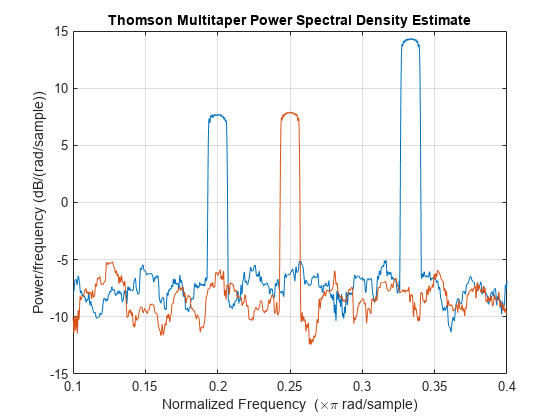
Repeat the computation, but now specify a sample rate of 2 kHz.
Fs = 2e3;

pmtm(x,{nw,ntp},w*(Fs/2),Fs)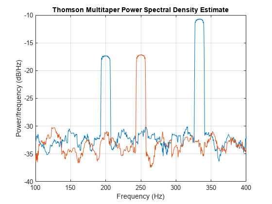
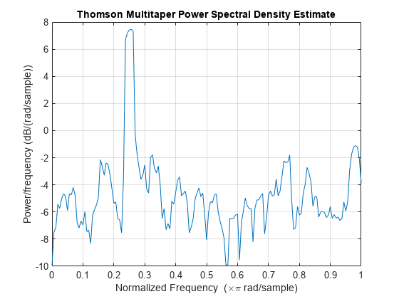
Obtain the multitaper PSD estimate with a specified time-halfbandwidth product.
Create a sine wave with an angular frequency of rad/sample with additive N(0,1) white noise. The signal is 320 samples in length. Obtain the multitaper PSD estimate with a time-halfbandwidth product of 2.5. The resolution bandwidth is rad/sample. The default number of DFT points is 512. Because the signal is real-valued, the PSD estimate is one-sided and there are 512/2+1 points in the PSD estimate.
rng("default")
n = 0:319;
x = cos(pi/4*n) + randn(size(n));
pmtm(x,2.5)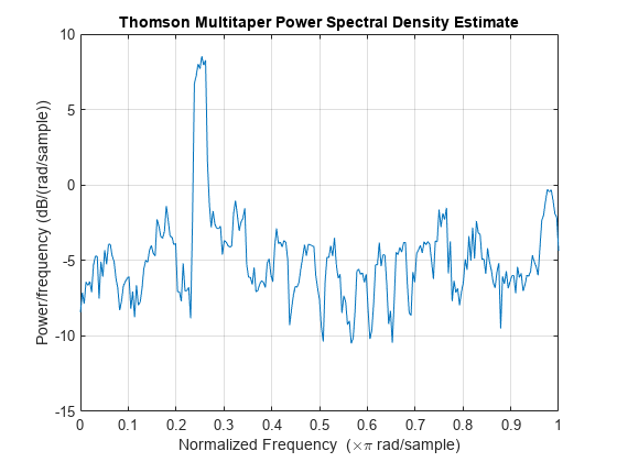
Obtain the multitaper PSD estimate of an input signal consisting of a discrete-time sinusoid with an angular frequency of rad/sample with additive N(0,1) white noise. Use a DFT length equal to the signal length.
Create a sine wave with an angular frequency of rad/sample with additive N(0,1) white noise. The signal is 320 samples in length. Obtain the multitaper PSD estimate with a time-halfbandwidth product of 3 and a DFT length equal to the signal length. Because the signal is real-valued, the one-sided PSD estimate is returned by default with a length equal to 320/2+1.
n = 0:319;
x = cos(pi/4*n) + randn(size(n));
pmtm(x,3,length(x))
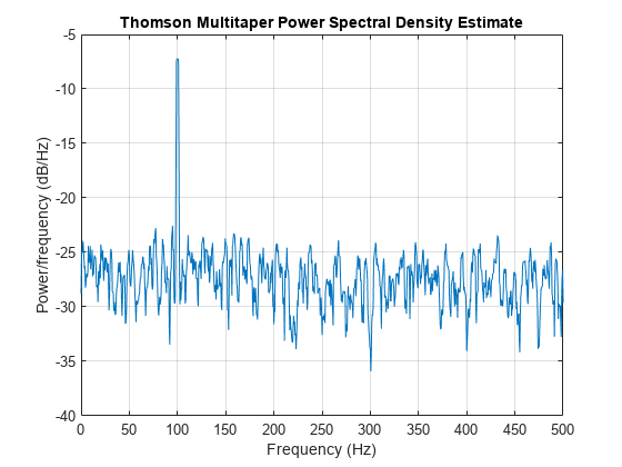
Obtain the multitaper PSD estimate of a signal sampled at 1 kHz. The signal is a 100 Hz sine wave in additive N(0,1) white noise. The signal duration is 2 s. Use a time-halfbandwidth product of 3 and DFT length equal to the signal length.
rng("default")
Fs = 1000;
t = 0:1/Fs:2-1/Fs;
x = cos(2*pi*100*t) + randn(size(t));
[pxx,f] = pmtm(x,3,length(x),Fs);
Plot the multitaper PSD estimate.
pmtm(x,3,length(x),Fs)
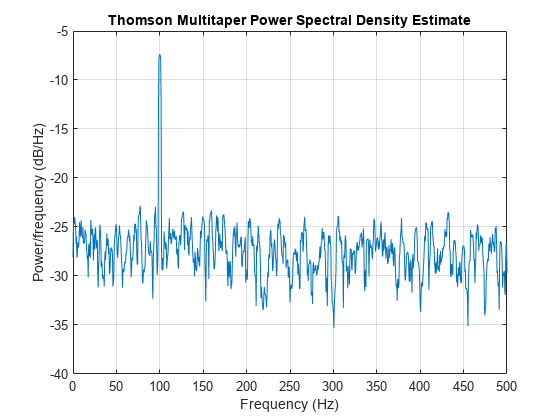
Obtain a multitaper PSD estimate where the individual tapered direct spectral estimates are given equal weight in the average.
Obtain the multitaper PSD estimate of a signal sampled at 1 kHz. The signal is a 100 Hz sine wave in additive N(0,1) white noise. The signal duration is 2 s. Use a time-halfbandwidth product of 3 and a DFT length equal to the signal length. Use the "unity" option to give equal weight in the average to each of the individual tapered direct spectral estimates.
rng("default")
Fs = 1000;
t = 0:1/Fs:2-1/Fs;
x = cos(2*pi*100*t) + randn(size(t));
[pxx,f] = pmtm(x,3,length(x),Fs,"unity");
Plot the multitaper PSD estimate.
pmtm(x,3,length(x),Fs,"unity")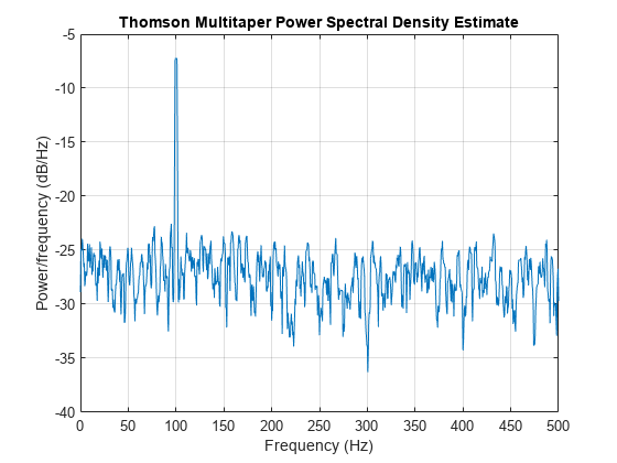
This example examines the frequency-domain concentrations of the DPSS sequences. The example produces a multitaper PSD estimate of an input signal by precomputing the Slepian sequences and selecting only those with more than 99% of their energy concentrated in the resolution bandwidth.
The signal is a 100 Hz sine wave in additive N(0,1) white noise. The signal duration is 2 seconds.
rng("default")
Fs = 1000;
t = 0:1/Fs:2-1/Fs;
x = cos(2*pi*100*t) + randn(size(t));
Set the time-half-bandwidth product to 3.5. For the signal length of 2000 samples and a sample rate of 1 kHz, the resolution bandwidth is [–1.75,1.75] Hz. Calculate the first 10 Slepian sequences and examine their frequency concentrations in the specified resolution bandwidth.
[e,v] = dpss(length(x),3.5,10);
lv = length(v);

stem(1:lv,v,"filled")
ylim([0 1.2])
title("Proportion of Energy in [-w,w] of k-th Slepian Sequence")
![Figure contains an axes object. The axes object with title Proportion of Energy in [-w,w] of k-th Slepian Sequence contains an object of type stem.](../../examples/signal/win64/DPSSSequencesAndTheirFrequencyDomainConcentrationsExample_01.png)
Determine the number of Slepian sequences with energy concentrations greater than 99%. Using the selected DPSS sequences, obtain the multitaper PSD estimate. Set DropLastTaper to false to use all the selected tapers.
hold on
plot([1 lv],0.99*[1 1])
hold off
![Figure contains an axes object. The axes object with title Proportion of Energy in [-w,w] of k-th Slepian Sequence contains 2 objects of type stem, line.](../../examples/signal/win64/DPSSSequencesAndTheirFrequencyDomainConcentrationsExample_02.png)
idx = find(v>0.99,1,"last")idx = 5
[pxx,f] = pmtm(x,e(:,1:idx),v(1:idx),length(x),Fs,DropLastTaper=false);
Plot the multitaper PSD estimate.
pmtm(x,e(:,1:idx),v(1:idx),length(x),Fs,DropLastTaper=false)
Obtain the multitaper PSD estimate of a 100 Hz sine wave in additive N(0,1) noise. The sample rate is 1 kHz. Use the "centered" option to obtain the DC-centered PSD.
rng("default")
Fs = 1000;
t = 0:1/Fs:2-1/Fs;
x = cos(2*pi*100*t) + randn(size(t));
[pxx,f] = pmtm(x,3.5,length(x),Fs,"centered");
Plot the DC-centered PSD estimate.
pmtm(x,3.5,length(x),Fs,"centered")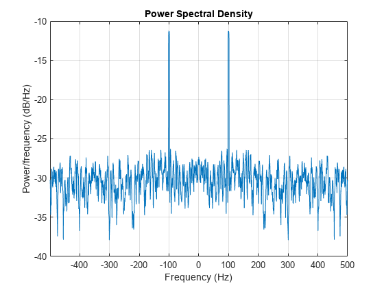
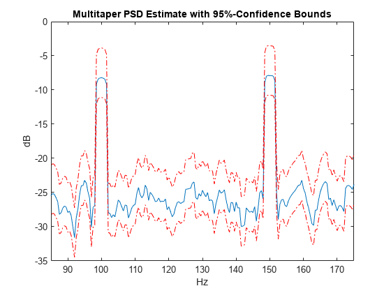
The following example illustrates the use of confidence bounds with the multitaper PSD estimate. While not a necessary condition for statistical significance, frequencies in the multitaper PSD estimate where the lower confidence bound exceeds the upper confidence bound for surrounding PSD estimates clearly indicate significant oscillations in the time series.
Create a signal consisting of the superposition of 100-Hz and 150-Hz sine waves in additive white N(0,1) noise. The amplitude of the two sine waves is 1. The sample rate is 1 kHz. The signal is 2 s in duration.
rng("default")
Fs = 1000;
t = 0:1/Fs:2-1/Fs;
x = cos(2*pi*100*t) + cos(2*pi*150*t) + randn(size(t));
Obtain the multitaper PSD estimate with 95%-confidence bounds.
[pxx,f,pxxc] = pmtm(x,3.5,length(x),Fs,ConfidenceLevel=0.95);
Plot the PSD estimate along with the confidence interval and zoom in on the frequency region of interest near 100 and 150 Hz. The lower confidence bound in the immediate vicinity of 100 and 150 Hz is significantly above the upper confidence bound outside the vicinity of 100 and 150 Hz.
plot(f,pow2db(pxx))
hold on
plot(f,pow2db(pxxc),"-.",Color=[0.866 0.329 0])
xlim([85 175])
xlabel("Hz")
ylabel("dB")
title("Multitaper PSD Estimate with 95%-Confidence Bounds")
Generate 1024 samples of a multichannel signal consisting of three sinusoids in additive white Gaussian noise. The sinusoids' frequencies are , , and rad/sample. Estimate the PSD of the signal using Thomson's multitaper method and plot it.
N = 1024;
n = 0:N-1;

w = pi./[2;3;4];

rng("default")
x = cos(w*n)' + randn(length(n),3);

pmtm(x)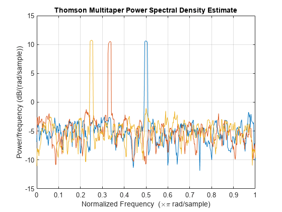
Input Arguments
Output Arguments
More About
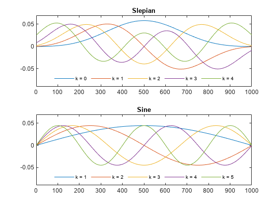
Generate the first five Slepian tapers corresponding to a time-halfbandwidth product of 3. Specify a taper length of 1000.
N = 1000;
nw = 3;
ns = 2*(nw)-1;

tprs = dpss(N,nw,ns);
lbs = "Slepian";
Generate the first five sine tapers.
n = 1:N;
k = 1:ns;

tprs(:,:,2) = sqrt(2/(N+1))*sin(pi*n'*k/(N+1));
lbs(2) = "Sine";
Plot the two sets of tapers.
for kj = 1:2
    subplot(2,1,kj)
    plot(tprs(:,:,kj))
    title(lbs(kj))
    legend("k = " + (k+kj-2), ...
        Orientation="horizontal",Location="south")
    legend("boxoff")
    ylim([-0.09 0.07])
end
References
[1] McCoy, Emma J., Andrew T. Walden, and Donald B. Percival. "Multitaper Spectral Estimation of Power Law Processes." IEEE® Transactions on Signal Processing 46, no. 3 (March 1998): 655–68. https://doi.org/10.1109/78.661333.
[2] Percival, Donald B., and Andrew T. Walden. Spectral Analysis for Physical Applications: Multitaper and Conventional Univariate Techniques. Cambridge; New York, NY, USA: Cambridge University Press, 1993.
[3] Riedel, Kurt S., and Alexander Sidorenko. “Minimum Bias Multiple Taper Spectral Estimation.” IEEE Transactions on Signal Processing 43, no. 1 (January 1995): 188–95. https://doi.org/10.1109/78.365298.
[4] Thomson, David J. "Spectrum estimation and harmonic analysis." Proceedings of the IEEE 70, no. 9 (1982): 1055–96. https://doi.org/10.1109/PROC.1982.12433.