periodogram
Periodogram power spectral density estimate
Syntax
Description
[
returns the periodogram PSD estimate of the signal pxx,f] = periodogram(x,win,freqSpec)x and
the frequencies f (rad/sample), where the
periodogram function:
Uses
winto divide the signal into segments and windows them.Computes the discrete Fourier transform (DFT) over the number of DFT points or at the frequencies specified in
freqSpec.
To use default values for any of these input arguments, specify
them as empty, [].
[
also specifies the frequency range and spectrum type for any of the previous
syntaxes. You can specify either or both of these input arguments.pxx,f] = periodogram(___,freqRange,spectrumType)
[
reassigns each PSD estimate or power spectrum estimate to the location of its
center of energy. The vector rpxx,f,pxx,fc] = periodogram(___,"reassigned")rpxx contains the sum of the
estimates reassigned to each element of f. This syntax also
returns the center-of-energy frequencies, fc.
If your signal contains well-localized spectral components, then the
"reassigned" argument generates a sharper
periodogram.
periodogram(___) with no output arguments
plots the periodogram PSD estimate or power spectrum in the current figure
window.
Examples
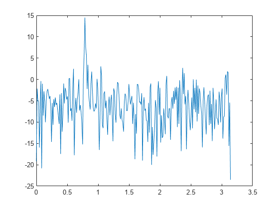
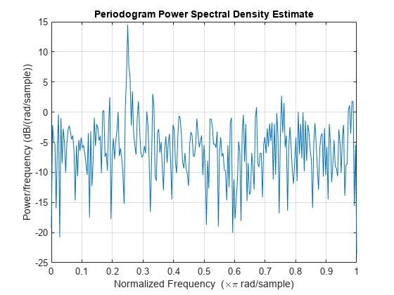
Obtain the periodogram of an input signal consisting of a discrete-time sinusoid with an angular frequency of rad/sample with additive white noise.
Create a sine wave with an angular frequency of rad/sample with additive white noise. The signal is 320 samples in length. Obtain the periodogram using the default rectangular window and DFT length. The DFT length is the next power of two greater than the signal length, or 512 points. Because the signal is real-valued and has even length, the periodogram is one-sided and there are 512/2+1 points.
n = 0:319;
x = cos(pi/4*n) + randn(size(n));
[pxx,w] = periodogram(x);
plot(w/pi,pow2db(pxx))
xlabel("Normalized Frequency (\times \pi rad/sample)")
title("Periodogram Power Spectral Density Estimate")
Repeat the plot using periodogram with no outputs.
periodogram(x)
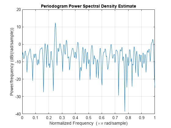
Obtain the modified periodogram of an input signal consisting of a discrete-time sinusoid with an angular frequency of radians/sample with additive white noise.
Create a sine wave with an angular frequency of radians/sample with additive white noise. The signal is 320 samples in length. Obtain the modified periodogram using a Hamming window and default DFT length. The DFT length is the next power of two greater than the signal length, or 512 points. Because the signal is real-valued and has even length, the periodogram is one-sided and there are 512/2+1 points.
n = 0:319;
x = cos(pi/4*n) + randn(size(n));
periodogram(x,hamming(length(x)))
Obtain the periodogram of an input signal consisting of a discrete-time sinusoid with an angular frequency of radians/sample with additive white noise. Use a DFT length equal to the signal length.
Create a sine wave with an angular frequency of radians/sample with additive white noise. The signal is 320 samples in length. Obtain the periodogram using the default rectangular window and DFT length equal to the signal length. Because the signal is real-valued, the one-sided periodogram is returned by default with a length equal to 320/2+1.
rng("default")
n = 0:319;
x = cos(pi/4*n) + randn(size(n));
nfft = length(x);
periodogram(x,[],nfft)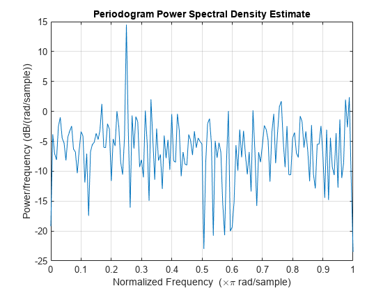
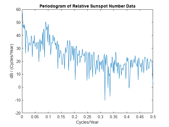
Obtain the periodogram of the Wolf (relative sunspot) number data sampled yearly between 1700 and 1987.
Load the relative sunspot number data. Obtain the periodogram using the default rectangular window and number of DFT points (512 in this example). The sample rate for these data is 1 sample/year.
load sunspot.dat
relNums=sunspot(:,2);

[pxx,f] = periodogram(relNums,[],[],1);
Plot the periodogram. There is a peak in the periodogram at approximately 0.1 cycles/year, which indicates a period of approximately 10 years.
plot(f,pow2db(pxx))
xlabel("Cycles/Year")
ylabel("dB / (Cycles/Year)")
title("Periodogram of Relative Sunspot Number Data")
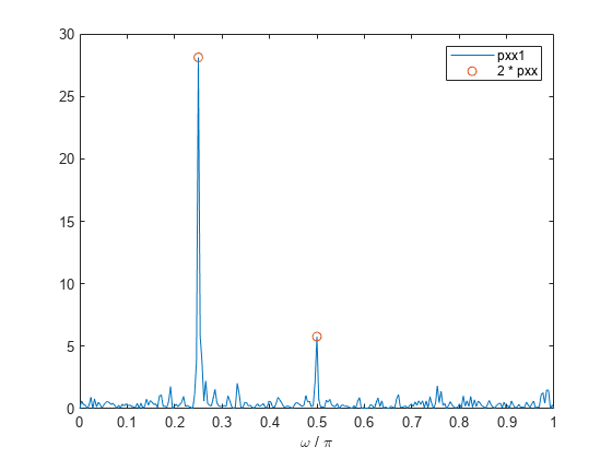
Obtain the periodogram of an input signal consisting of two discrete-time sinusoids with an angular frequencies of and rad/sample in additive white noise. Obtain the two-sided periodogram estimates at and rad/sample.
n = 0:319;
x = cos(pi/4*n) + 0.5*sin(pi/2*n) + randn(size(n));

[pxx,w] = periodogram(x,[],[pi/4 pi/2]);
pxx
pxx = 1×2

   14.0589    2.8872
[pxx1,w1] = periodogram(x);
Compare the result to the one-sided periodogram. The periodogram values obtained are 1/2 the values in the one-sided periodogram. When you evaluate the periodogram at a specific set of frequencies, the output is a two-sided estimate.
plot(w1/pi,pxx1,w/pi,2*pxx,"o")
legend("pxx1","2*pxx")
xlabel("Normalized Frequency (\times \pi rad/sample)")
title("Periodogram Power Spectral Density Estimate")
Create a signal consisting of two sine waves with frequencies of 100 and 200 Hz in N(0,1) white additive noise. The sample rate is 1 kHz. Obtain the two-sided periodogram at 100 and 200 Hz.
rng("default")
Fs = 1000;
t = 0:0.001:1-0.001;
x = cos(2*pi*100*t) + sin(2*pi*200*t) + randn(size(t));

freq = [100 200];
pxx = periodogram(x,[],freq,Fs)
pxx = 1×2
0.2647 0.2313
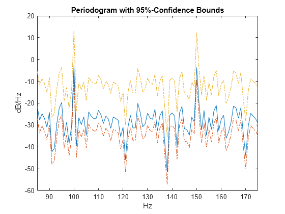
This example illustrates the use of confidence bounds with the periodogram. While not a necessary condition for statistical significance, frequencies in the periodogram where the lower confidence bound exceeds the upper confidence bound for surrounding PSD estimates clearly indicate significant oscillations in the time series.
Create a signal consisting of the superposition of 100 Hz and 150 Hz sine waves in additive white N(0,1) noise. The amplitude of the two sine waves is 1. The sample rate is 1 kHz.
rng("default")
Fs = 1000;
t = 0:1/Fs:1-1/Fs;
x = cos(2*pi*100*t) + sin(2*pi*150*t) + randn(size(t));
Obtain the periodogram PSD estimate with 95%-confidence bounds.
L = length(x);
[pxx,f,pxxc] = periodogram(x,rectwin(L),L,Fs,ConfidenceLevel=0.95);
Plot the periodogram along with the confidence interval and zoom in on the frequency region of interest near 100 and 150 Hz. The lower confidence bound in the immediate vicinity of 100 and 150 Hz is significantly above the upper confidence bound outside the vicinity of 100 and 150 Hz.
plot(f,pow2db(pxx))
hold on
plot(f,pow2db(pxxc),"-.",Color=[0.866 0.329 0])

xlim([85 175])
xlabel("Hz")
ylabel("dB/Hz")
title("Periodogram with 95%-Confidence Bounds")
Obtain the periodogram of a 100 Hz sine wave in additive noise. The sample rate is 1 kHz. Use the "centered" option to obtain the DC-centered periodogram and plot the result.
fs = 1000;
t = 0:0.001:1-0.001;
x = cos(2*pi*100*t)+randn(size(t));
periodogram(x,[],length(x),fs,"centered")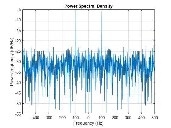
Generate a signal that consists of a 200 Hz sinusoid embedded in white Gaussian noise. The signal is sampled at 1 kHz for 1 second. The noise has a variance of 0.01². Reset the random number generator for reproducible results.
rng("default")

Fs = 1000;
t = 0:1/Fs:1-1/Fs;
N = length(t);
x = sin(2*pi*t*200) + 0.01*randn(size(t));
Use the FFT to compute the power spectrum of the signal, normalized by the signal length. The sinusoid is in-bin, so all the power is concentrated in a single frequency sample. Plot the one-sided spectrum. Zoom in to the vicinity of the peak.
q = fft(x,N);
ff = 0:Fs/N:Fs-Fs/N;

ffts = q*q'/N^2
ffts =
0.4997
ff = ff(1:floor(N/2)+1);
q = q(1:floor(N/2)+1);

stem(ff,abs(q)/N,"*")
axis([190 210 0 0.55])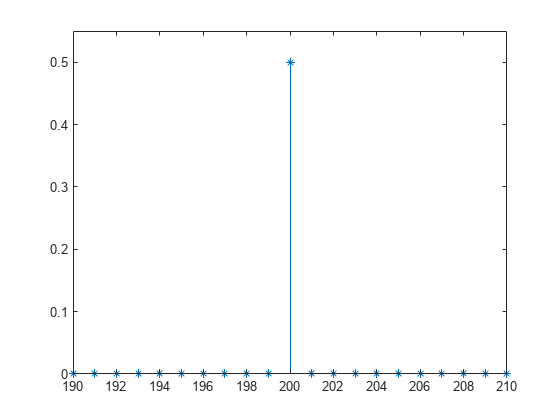
Use periodogram to compute the power spectrum of the signal. Specify a Hann window and an FFT length of 1024. Find the percentage difference between the estimated power at 200 Hz and the actual value.
wind = hann(N);

[pun,fr] = periodogram(x,wind,1024,Fs,"power");

hold on
stem(fr,pun)
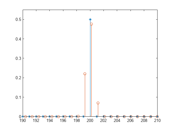
periodogErr = abs(max(pun)-ffts)/ffts*100
periodogErr =
4.7349
Recompute the power spectrum, but this time use reassignment. Plot the new estimate and compare its maximum with the FFT value.
[pre,ft,pxx,fx] = periodogram(x,wind,1024,Fs,"power","reassigned");

stem(fx,pre)
hold off
legend(["Original" "Periodogram" "Reassigned"])
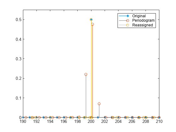
reassignErr = abs(max(pre)-ffts)/ffts*100
reassignErr =
0.0779
Estimate the power of sinusoid at a specific frequency using the "power" option.
Create a 100 Hz sinusoid one second in duration sampled at 1 kHz. The amplitude of the sine wave is 1.8, which equates to a power of 1.8²/2 = 1.62. Estimate the power using the "power" option.
fs = 1000;
t = 0:1/fs:1-1/fs;
x = 1.8*cos(2*pi*100*t);
[pxx,f] = periodogram(x,hamming(length(x)),length(x),fs,"power");
[pwrest,idx] = max(pxx);
fprintf("The maximum power occurs at %3.1f Hz\n",f(idx))
The maximum power occurs at 100.0 Hz
fprintf("The power estimate is %2.2f\n",pwrest)The power estimate is 1.62
Generate 1024 samples of a multichannel signal consisting of three sinusoids in additive white Gaussian noise. The sinusoids frequencies are , , and rad/sample. Estimate the PSD of the signal using the periodogram and plot it.
rng("default")
N = 1024;
n = 0:N-1;

w = pi./[2;3;4];
x = cos(w*n)' + randn(length(n),3);

periodogram(x)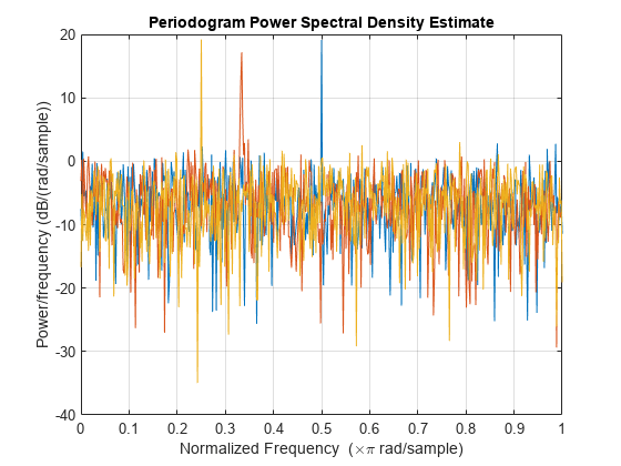
Examine the function myPeriodogram.m that returns the Modified Periodogram power spectral density (PSD) estimate of an input signal using a window. The function specifies a number of discrete Fourier transform points equal to the length of the input signal.
type myPeriodogramfunction [pxx,f] = myPeriodogram(inputData,window) %#codegen
nfft = length(inputData);
[pxx,f] = periodogram(inputData,window,nfft);
end
Use codegen (MATLAB Coder) to generate a MEX function.
The
%#codegendirective in the function indicates that the MATLAB® code is intended for code generation.The
-argsoption specifies example arguments that define the size, class, and complexity of the inputs to the MEX-file. For this example, specifyinputDataas a 1024-by-1 double precision random vector andwindowas a Hamming window of length 1024. In subsequent calls to the MEX function, use 1024-sample input signals and windows.To set a different name for the MEX function, use the
-ooption.To generate a code generation report, add the
-reportoption at the end of thecodegencommand.
codegen myPeriodogram -args {randn(1024,1),hamming(1024)}
Code generation successful.
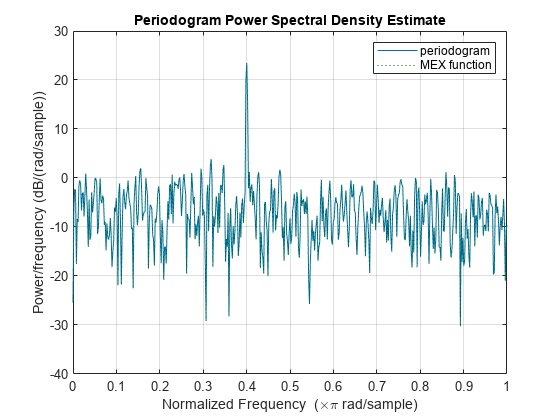
Compute the PSD estimate of a 1024-sample noisy sinusoid using the periodogram function and the generated MEX function. Specify a sinusoid normalized frequency of rad/sample and a Hann window. Plot the two estimates to verify that they coincide.
N = 1024;
x = 2*cos(2*pi/5*(0:N-1)') + randn(N,1);
periodogram(x,hann(N))
[pxMex,fMex] = myPeriodogram_mex(x,hann(N));
hold on
plot(fMex/pi,pow2db(pxMex),"--")
hold off
grid on
legend(["periodogram" "MEX function"])
Since R2026a
Plot the periodogram power spectral density (PSD) estimate and periodogram power spectrum for four signals in the specified target axes and panel containers.
Create four oscillating signals with a sample rate of 10 kHz for three seconds.
Fs = 10e3;
t = 0:1/Fs:3;
x1 = sinc(Fs/2.5*(t-mean(t)));
x2 = sum(cos(2*pi*600*[1 3 5 7]'.*t),1) + randn(size(t))/1e4;
x3 = exp(1j*pi*sin(4*t)*Fs/10);
x4 = chirp(t,Fs/10,t(end),Fs/2.5,"quadratic");
Plot Periodogram PSD Estimate and Power Spectrum in Target Axes
Create two axes in the southwestern and northeastern corners of a new figure window.
fig = figure;
ax1 = axes(fig,Position=[0.09 0.1 0.60 0.45]);
ax2 = axes(fig,Position=[0.50 0.7 0.47 0.25]);
Plot the periodogram PSD estimate and power spectrum of the signals x1 and x2 in the southwestern and northeastern axes of the figure, respectively. Use a Kaiser window and 512 DFT points.
g = kaiser(length(t),5);
nfft = 512;

periodogram(x1,g,nfft,Fs,Parent=ax1)
periodogram(x2,g,nfft,Fs,"power",Parent=ax2)
Plot Periodogram PSD Estimate in Target UI Axes
Create an axes in the northwestern corner of a new UI figure window.
uif = uifigure(Position=[100 100 720 540]);
ax3 = uiaxes(uif,Position=[5 305 300 200]);
Plot the periodogram PSD estimate of the signal x3 on the figure axes. Display the frequencies centered at 0 kHz.
periodogram(x3,g,nfft,Fs,"centered",Parent=ax3)
title(ax3,"Periodogram in UI Axes")

Plot Reassigned Periodogram PSD Estimate in Target Panel Container
Add a panel container in the southeastern corner of the UI figure window.
p = uipanel(uif,Position=[300 5 400 325], ...
    Title="Periodogram in Panel Container", ...
    BackgroundColor="white");
Plot the reassigned periodogram PSD estimate of the signal x4 on the panel container.
periodogram(x4,g,nfft,Fs,"reassigned",Parent=p)
Input Arguments
Input signal, specified as a vector or as a matrix. If you specify x as a
matrix, then periodogram treats its columns as independent
channels.
Example: cos(pi/4*(0:159))+randn(1,160) is
a single-channel row-vector signal.
Example: cos(pi./[4;2]*(0:159))'+randn(160,2) is
a two-channel signal.
Data Types: single | double
Complex Number Support: Yes
Window, specified as a row or column vector with the same length as the
input signal. If you specify win as empty, then
periodogram uses a rectangular window. If you
specify the "reassigned" option and an empty
win, then the function uses a Kaiser window with β = 38.
Note
The default rectangular window has a 13.3 dB sidelobe attenuation, which may mask spectral content below this value (relative to the peak spectral content). Choosing different windows enables you to make tradeoffs between resolution (for example, using a rectangular window) and sidelobe attenuation (for example, using a Hann window). See Window Designer for more details.
Data Types: single | double
Frequency specification, specified as one of these values:
Empty,
[]—periodogramcalculates the spectral estimates using a number of DFT points equal to the greater of 256 or the next power of two that is equal or larger than the window length.Positive integer —
periodogramcalculates the spectral estimates using the number of DFT points specified in this argument.If
freqSpecis greater than the segment length, thenperiodogrampads the segment data with zeros.If
freqSpecis less than the segment length, thenperiodogrampartitions the segment modulofreqSpecand sums the resulting segment frames.
Vector of at least two elements —
periodogramcalculates the spectral estimates at the frequencies specified infreqSpec.If you specify the sample rate,
Fs,periodogramassumesfreqSpecas cyclical frequencies in the same units as ofFs.If you do not specify
Fs,periodogramassumesfreqSpecas normalized frequencies in rad/sample.
Example: freqSpec = 512 specifies 512 DFT points.
Example: freqSpec = pi./[8 4 2] specifies a vector of three normalized frequencies.
Data Types: single | double
Sample rate, specified as a positive scalar. The sample rate is the number of samples per unit time. If the unit of time is seconds, then the sample rate is in Hz.
If you specify
Fsas empty[], thenperiodogramassumes that the input signalxhas a sample rate of 1 Hz.If you do not specify
Fs, thenperiodogramassumes that the input signalxhas a sample rate of 2π rad/sample.
Frequency range of the PSD estimate or power spectrum, specified as
"onesided", "twosided", or
"centered".
The periodogram function returns
pxx with a number of rows and frequency interval
that depends on the value specified in freqRange,
whether the number of DFT points freqSpec is even or
odd, and whether Fs is specified or not.
freqRange | freqSpec | Number of Rows in
pxx | Frequency Interval for
| |
|---|---|---|---|---|
|
| |||
"onesided"(default if x is real-valued) | Even | freqSpec/2 + 1 | [0,π] rad/sample | [0,Fs/2] cycles/unit
time |
| Odd | (freqSpec + 1)/2 | [0,π) rad/sample | [0,Fs/2) cycles/unit
time | |
"twosided"(default if x is complex-valued) | Even or odd | freqSpec | [0,2π) rad/sample | [0,Fs) cycles/unit time |
"centered" | Even | freqSpec | (–π,π] rad/sample | (–Fs/2,Fs/2]
cycles/unit time |
| Odd | (–π,π) rad/sample | (–Fs/2,Fs/2)
cycles/unit time | ||
Note
This argument is not supported if you specify
freqSpecas a vector of cyclical or normalized frequencies.If you specify the
"onesided"value,periodogrammultiplies the power by 2 at all frequencies except 0 and the Nyquist frequency to conserve the total power.The
"onesided"value is not supported ifxis complex-valued.
Data Types: char | string
Power spectrum scaling, specified as one of these values:
"psd"—periodogramreturns the power spectral density."power"—periodogramscales each estimate of the PSD by the equivalent noise bandwidth of the window and returns an estimate of the power at each frequency. If you also specify"reassigned",periodogramintegrates the PSD over the width of each frequency bin before reassigning.
This table shows the scaling relation between the PSD
estimate and power spectrum estimate, either of both returned in
pxx, given an input signal x,
window vector win, frequency specification
freqSpec, and sample rate
Fs.
| Sample Rate | Scaling relation |
|---|---|
Fs specified | [~,~,~,psd] = periodogram(x,win,freqSpec,Fs,"psd"); [~,~,~,pow] = periodogram(x,win,freqSpec,Fs,"power"); pow is equivalent to
psd*enbw(win,Fs). |
Fs unspecified | [~,~,~,psd] = periodogram(x,win,freqSpec,"psd"); [~,~,~,pow] = periodogram(x,win,freqSpec,"power"); pow is equivalent to
psd*enbw(win,2*pi). |
Data Types: char | string
Coverage probability for the PSD estimate, specified as a scalar in the range (0,1).
If you specify ConfidenceLevel=p and pxxc,
the function outputs pxxc with the lower and upper bounds of the
p × 100% interval estimate for the true
PSD.
Since R2026a
Target parent container, specified as an Axes object, a
UIAxes object,
or a Panel
object.
If you specify Parent=h, the
periodogram function plots the periodogram PSD
estimate or power spectrum on the specified target parent container, whether
you call the function with or without output arguments.
For more information about target containers and the parent-child
relationship in MATLAB® graphics, see Graphics Object Hierarchy. For
more information about using Parent in
UIAxes and Panel objects to design
apps, see Plot Spectral Representations of Signal in App Designer.
Example: h = axes(figure,Position=[0.1 0.1 0.6 0.5])
defines an axes parent container. When you specify
periodogram(x,[],[],[],Parent=h), the function
plots the periodogram PSD of the input signal x in
the parent container h.
Output Arguments
PSD estimate or power spectrum, returned as a real-valued, nonnegative column vector or matrix.
Each column of
pxxis the PSD estimate or the or power spectrum of the corresponding column ofxand depending on how you specifyspectrumType.The units of the PSD estimate are in squared-magnitude units of the input signal per unit frequency. For example, if the input data
xis in volts, you specify the sample rateFsin hertz, and you assume a resistance of 1 Ω, then the PSD estimate is in watts per hertz.The units of the power spectrum are in squared-magnitude units of the input signal. For example, if the input data
xis in volts and you assume a resistance of 1 Ω, then the PSD estimate is in watts.
Frequencies associated with the PSD estimate, returned as a real-valued column vector.
If you specify
Fs, thenfcontains cyclical frequencies in Hz.If you do not specify
Fs, thenfcontains normalized frequencies in rad/sample.
Confidence bounds, returned as a real-valued matrix.
pxxchas the same number of rows as inpxx.pxxchas twice as many columns aspxx.Odd-numbered columns contain the lower bounds of the confidence intervals.
Even-numbered columns contain the upper bounds of the confidence intervals.
Thus,
pxxc(m,2*n-1)is the lower confidence bound andpxxc(m,2*n)is the upper confidence bound corresponding to the estimatepxx(m,n).The coverage probability of the confidence intervals is determined by the value of the
pinput.
Data Types: single | double
Reassigned PSD estimate, returned as a real-valued, nonnegative column
vector or matrix. Each column of rpxx is the reassigned
PSD estimate of the corresponding column of x.
Center-of-energy frequencies, returned as a vector or matrix.
More About
The periodogram is a nonparametric estimate of the power spectral
density (PSD) of a wide-sense stationary random process. The periodogram is the
Fourier transform of the biased estimate of the autocorrelation sequence. For a
signal xn sampled at
Fs samples per unit time, the periodogram is defined as
where Δt is the sampling interval. For a one-sided periodogram, the values at all frequencies except 0 and the Nyquist, 1/2Δt, are multiplied by 2 so that the total power is conserved.
If the frequencies are in radians per sample, the periodogram is defined as
The frequency range in the preceding equations has variations depending on the
value of the freqRange argument. See the description of
freqRange in Input Arguments.
The integral of the true PSD, P(f), over one period, 1/Δt for cyclical frequency and 2π for normalized frequency, is equal to the variance of the wide-sense stationary random process:
For normalized frequencies, replace the limits of integration appropriately.
The modified periodogram multiplies the input time series by a window function. A suitable window function is nonnegative and decays to zero at the beginning and end points. Multiplying the time series by the window function tapers the data gradually on and off and helps to alleviate the leakage in the periodogram. See Bias and Variability in the Periodogram for an example.
If hn is a window function, the modified periodogram is defined by
where Δt is the sampling interval.
If the frequencies are in radians per sample, the modified periodogram is defined as
The frequency range in the preceding equations has variations depending on the
value of the freqRange argument. See the description of
freqRange in Input Arguments.
The reassignment technique sharpens the localization of spectral estimates and produces periodograms that are easier to read and interpret. This technique reassigns each PSD estimate to the center of energy of its bin, away from the bin’s geometric center. It provides exact localization for chirps and impulses.
References
[1] Auger, François, and Patrick Flandrin. "Improving the Readability of Time-Frequency and Time-Scale Representations by the Reassignment Method." IEEE® Transactions on Signal Processing. Vol. 43, May 1995, pp. 1068–1089.
[2] Fulop, Sean A., and Kelly Fitz. "Algorithms for computing the time-corrected instantaneous frequency (reassigned) spectrogram, with applications." Journal of the Acoustical Society of America. Vol. 119, January 2006, pp. 360–371.
Extended Capabilities
C/C++ Code Generation
Generate C and C++ code using MATLAB® Coder™.
GPU Code Generation
Generate CUDA® code for NVIDIA® GPUs using GPU Coder™.
This function fully supports GPU arrays. For more information, see Run MATLAB Functions on a GPU (Parallel Computing Toolbox).
Version History
Introduced before R2006aThe periodogram function supports plotting output in a parent
axes or panel container specified using the Parent input
argument.
The periodogram function supports single-precision
variable-size window inputs for code generation.
The periodogram function supports code generation for
graphical processing units (GPUs). You must have MATLAB
Coder™ and GPU Coder™ to generate CUDA® code.
The periodogram function supports single-precision
inputs.
You can now use the Create
Plot Live Editor task to visualize the output of
periodogram interactively. You can select different chart
types and set optional parameters. The task also automatically generates code that
becomes part of your live script.
MATLAB Command
You clicked a link that corresponds to this MATLAB command:
Run the command by entering it in the MATLAB Command Window. Web browsers do not support MATLAB commands.
Select a Web Site
Choose a web site to get translated content where available and see local events and offers. Based on your location, we recommend that you select: .
You can also select a web site from the following list
How to Get Best Site Performance
Select the China site (in Chinese or English) for best site performance. Other MathWorks country sites are not optimized for visits from your location.
Americas
- América Latina (Español)
- Canada (English)
- United States (English)
Europe
- Belgium (English)
- Denmark (English)
- Deutschland (Deutsch)
- España (Español)
- Finland (English)
- France (Français)
- Ireland (English)
- Italia (Italiano)
- Luxembourg (English)
- Netherlands (English)
- Norway (English)
- Österreich (Deutsch)
- Portugal (English)
- Sweden (English)
- Switzerland
- United Kingdom (English)