sfdr
Spurious free dynamic range
Syntax
Description
r = sfdr(x)r, in
dB of the real sinusoidal signal, x. sfdr computes
the power spectrum using a modified periodogram and a Kaiser window
with β = 38. The mean is subtracted from x before
computing the power spectrum. The number of points used in the computation
of the discrete Fourier transform (DFT) is the same as the length
of the signal, x.
r = sfdr(x,fs,msd)msd,
specified in cycles/unit time. The sample rate is fs.
If the carrier frequency is Fc, then all spurs
in the interval (Fc-msd, Fc+msd)
are ignored.
r = sfdr(sxx,f,'power')sxx. f is
the vector of frequencies corresponding to the power estimates in sxx.
The first element of f must equal 0. The algorithm
removes all the power that decreases monotonically away from the DC
bin.
r = sfdr(sxx,f,msd,'power')msd.
If the carrier frequency is Fc, then all spurs
in the interval (Fc-msd, Fc+msd)
are ignored. When the input to sfdr is a power
spectrum, specifying msd can prevent high sidelobe
levels from being identified as spurs.
sfdr(___) with no output arguments
plots the spectrum of the signal in the current figure window. It
uses different colors to draw the fundamental component, the DC value,
and the rest of the spectrum. It shades the SFDR and displays its
value above the plot. It also labels the fundamental and the largest
spur.
Examples
SFDR of Sinusoid
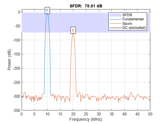
Obtain the SFDR for a 10 MHz tone with amplitude 1 sampled at 100 MHz. There is a spur at the 1st harmonic (20 MHz) with an amplitude of .
deltat = 1e-8;
fs = 1/deltat;
t = 0:deltat:1e-5-deltat;
x = cos(2*pi*10e6*t)+3.16e-4*cos(2*pi*20e6*t);
r = sfdr(x,fs)
r = 70.0063
Display the spectrum of the signal. Annotate the fundamental, the DC value, the spur, and the SFDR.
sfdr(x,fs);
Minimum Spur Distance
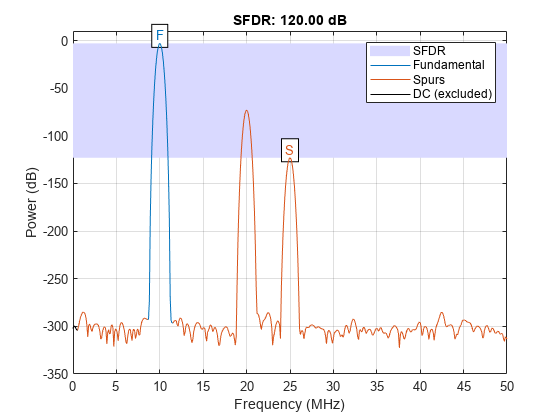
Obtain the SFDR for a 10 MHz tone with amplitude 1 sampled at 100 MHz. There is a spur at the 1st harmonic (20 MHz) with an amplitude of and another spur at 25 MHz with an amplitude of . Skip the first harmonic by using a minimum spur distance of 11 MHz.
deltat = 1e-8;
fs = 1/deltat;
t = 0:deltat:1e-5-deltat;
x = cos(2*pi*10e6*t)+3.16e-4*cos(2*pi*20e6*t)+ ...
    0.1e-5*cos(2*pi*25e6*t);
r = sfdr(x,fs,11e6)
r = 120.0000
Display the spectrum of the signal. Annotate the fundamental, the DC value, the spurs, and the SFDR.
sfdr(x,fs,11e6);
SFDR from Periodogram
Obtain the power spectrum of a 10 MHz tone with amplitude 1 sampled at 100 MHz. There is a spur at the 1st harmonic (20 MHz) with an amplitude of . Use the one-sided power spectrum and a vector of corresponding frequencies in Hz to compute the SFDR.
deltat = 1e-8;
fs = 1/deltat;
t = 0:deltat:1e-6-deltat;
x = cos(2*pi*10e6*t)+3.16e-4*cos(2*pi*20e6*t);
[sxx,f] = periodogram(x,rectwin(length(x)),length(x),fs,'power');
r = sfdr(sxx,f,'power');
Display the spectrum of the signal. Annotate the fundamental, the DC value, the first spur, and the SFDR.
sfdr(sxx,f,'power');
Frequency and Power of Largest Spur
Determine the frequency in MHz for the largest spur. The input signal is a 10 MHz tone with amplitude 1 sampled at 100 MHz. There is a spur at the first harmonic (20 MHz) with an amplitude of .
deltat = 1e-8;
t = 0:deltat:1e-6-deltat;
x = cos(2*pi*10e6*t)+3.16e-4*cos(2*pi*20e6*t);
[r,spurpow,spurfreq] = sfdr(x,1/deltat);
spur_MHz = spurfreq/1e6
spur_MHz = 20
SFDR from Time Series
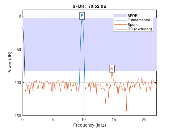
Create a superposition of three sinusoids, with frequencies of 9.8, 14.7, and 19.6 kHz, in white Gaussian additive noise. The signal is sampled at 44.1 kHz. The 9.8 kHz sine wave has an amplitude of 1 volt, the 14.7 kHz wave has an amplitude of 100 microvolts, and the 19.6 kHz signal has amplitude 30 microvolts. The noise has 0 mean and a variance of 0.01 microvolt. Additionally, the signal has a DC shift of 0.1 volt.
rng default

Fs = 44.1e3;
f1 = 9.8e3;
f2 = 14.7e3;
f3 = 19.6e3;
N = 900;

nT = (0:N-1)/Fs;
x = 0.1+sin(2*pi*f1*nT)+100e-6*sin(2*pi*f2*nT) ...
    +30e-6*sin(2*pi*f3*nT)+sqrt(1e-8)*randn(1,N);
Plot the spectrum and SFDR of the signal. Display its fundamental and its largest spur. The DC level is excluded from the SFDR computation.
sfdr(x,Fs);
Input Arguments
Output Arguments
More About
Extended Capabilities
Version History
Introduced in R2013a
You can also select a web site from the following list:
Americas
- América Latina (Español)
- Canada (English)
- United States (English)
Europe
- Belgium (English)
- Denmark (English)
- Deutschland (Deutsch)
- España (Español)
- Finland (English)
- France (Français)
- Ireland (English)
- Italia (Italiano)
- Luxembourg (English)
- Netherlands (English)
- Norway (English)
- Österreich (Deutsch)
- Portugal (English)
- Sweden (English)
- Switzerland
- United Kingdom (English)