pulseperiod
Period of bilevel pulse
Syntax
Description
p = pulseperiod(x)x. To determine the transitions for each pulse, the
pulseperiod function estimates the state levels of the input waveform by a
histogram method and identifies all regions which cross the upper-state boundary of the low
state and the lower-state boundary of the high state.
[
returns the mid-reference level instants p,initcross,finalcross]
= pulseperiod(___)finalcross of the final transition
of each pulse. You can specify an input combination from any of the previous syntaxes.
[
returns the mid-reference level instants p,initcross,finalcross,nextcross]
= pulseperiod(___)nextcross of the next detected
transition after each pulse.
[
returns the mid-reference level p,initcross,finalcross,nextcross,midlev]
= pulseperiod(___)midlev.
[
returns the pulse periods with additional options specified by one or more name-value
arguments.p,initcross,finalcross,nextcross,midlev]
= pulseperiod(___,Name,Value)
pulseperiod(___) plots the signal and darkens every other
identified pulse. The function marks the location of the mid crossings and their associated
reference level. The function also plots the state levels and their associated lower and upper
boundaries. You can adjust the boundaries using the 'Tolerance' name-value
argument.
Examples
Pulse Period of Bilevel Waveform
Compute the pulse period of a bilevel waveform with two positive-polarity transitions. The sample rate is 4 MHz.
load('pulseex.mat','x','t')

p = pulseperiod(x,t)
p = 5.0030e-06
Annotate the pulse period on a plot of the waveform.
pulseperiod(x,t);

Mid-Reference Level Instants of Pulse Period
Determine the mid-reference level instants that define the pulse period for a bilevel waveform.
load('pulseex.mat','x','t')
[~,initcross,~,nextcross] = pulseperiod(x,t)
initcross = 3.1240e-06
nextcross = 8.1270e-06
Output the pulse period. Mark the mid-reference level instants on a plot of the data.
pulseperiod(x,t)

ans = 5.0030e-06
Input Arguments
Output Arguments
More About
Pulse Polarity
If the initial transition of a pulse is positive-going, the pulse has positive polarity. This figure shows a positive-polarity pulse.

Equivalently, a positive-polarity (positive-going) pulse has a terminating state more positive than the originating state.
If the initial transition of a pulse is negative-going, the pulse has negative polarity. This figure shows a negative-polarity pulse.

Equivalently, a negative-polarity (negative-going) pulse has a originating state more positive than the terminating state.
State-Level Tolerances
You can specify lower- and upper-state boundaries for each state level. Define the boundaries as the state level plus or minus a scalar multiple of the difference between the high state and the low state. To provide a useful tolerance region, specify the scalar as a small number such as 2/100 or 3/100. In general, the  region for the low state is defined as
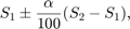
where  is the low-state level and
  is the high-state level. Replace the first term in the equation with to obtain the tolerance region for the high state.
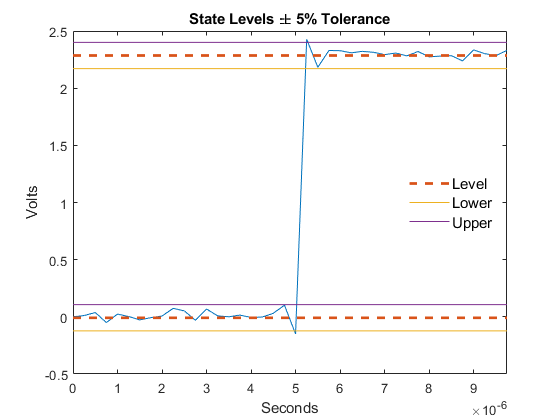
This figure shows lower and upper 5% state boundaries (tolerance regions) for a positive-polarity bilevel waveform. The thick dashed lines indicate the estimated state levels.
References
[1] IEEE® Standard on Transitions, Pulses, and Related Waveforms, IEEE Standard 181, 2003.
Extended Capabilities
Version History
Introduced in R2012a
See Also
You can also select a web site from the following list:
Americas
- América Latina (Español)
- Canada (English)
- United States (English)
Europe
- Belgium (English)
- Denmark (English)
- Deutschland (Deutsch)
- España (Español)
- Finland (English)
- France (Français)
- Ireland (English)
- Italia (Italiano)
- Luxembourg (English)
- Netherlands (English)
- Norway (English)
- Österreich (Deutsch)
- Portugal (English)
- Sweden (English)
- Switzerland
- United Kingdom (English)