anova
Description
An anova object contains the results of a one-, two-, or N-way
ANOVA. Use the properties of an anova object to determine if the
means in a set of response data differ with respect to the values (levels) of a factor or
multiple factors. The object properties include information about the coefficient estimates,
ANOVA model fit to the response data, and factors used to perform the analysis.
Creation
Syntax
Description
aov = anova(y)anova object aov for
the response data in the matrix y. Each column of
y is treated as a different factor value.
aov = anova(tbl,responseVarName)tbl as factors and response data. The
responseVarName argument specifies which variable contains the
response data.
aov = anova(tbl,formula)formula use only the variable names in
tbl.
aov = anova(___,Name=Value)
Input Arguments
Response data, specified as a matrix or a numeric vector.
If
yis a matrix,anovatreats each column ofyas a separate factor value in a one-way ANOVA. In this design, the function evaluates whether the population means of the columns are equal. Use this design when you want to perform a one-way ANOVA on data that is equally divided between each group (balanced ANOVA).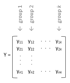
If
yis a numeric vector, you must also specify either thefactorsortblinput argument. For a one-way ANOVA,factorsis a cell array of character vectors or a vector in which each element represents the factor value of the corresponding element iny.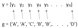
For an N-way ANOVA,
factorsis a cell array of vectors in which each cell is treated as a separate factor. Alternatively, for an N-way ANOVA, you can provide a tabletblin which each variable is treated as a separate factor. Use this design when you want to perform a two- or N-way ANOVA, or when factor values correspond to different numbers of observations iny(unbalanced ANOVA).
Note
The anova function ignores NaN
values, <undefined> values, empty characters, and empty
strings in y. If factors or
tbl contains NaN or
<undefined> values, or empty characters or strings, the
function ignores the corresponding observations in y. The ANOVA
is balanced if each factor value has the same number of observations after the
function disregards empty or NaN values. Otherwise, the function
performs an unbalanced ANOVA.
Data Types: single | double
Factors and factor values for the ANOVA, specified as a numeric, logical, categorical, string, or character vector, or a cell array of vectors. Factors and factor values are sometimes called grouping variables and group names, respectively.
For a one-way ANOVA, factors is a vector or cell array of
character vectors in which each element represents the factor value of the observation
in y at the same position. The anova
function groups observations in y by their factor values during
the ANOVA. The length of factors must be the same as the length
of y.
For a two- or N-way ANOVA, factors is a cell array of vectors
in which each cell corresponds to a different factor. Each vector contains the values
of the corresponding factor and must have the same length as y.
Factor values are associated with observations in y by their
index.
If factors contains NaN values,
anova ignores the corresponding observations in
y.
For more information on factors, see Grouping Variables.
Note
If factors or tbl contains
NaN values, <undefined> values, empty
characters, or empty strings, the anova function ignores the
corresponding observations in y. The ANOVA is balanced if each factor
value has the same number of observations after the function disregards empty or
NaN values. Otherwise, the function performs an unbalanced
ANOVA.
Example: [1,2,1,3,1,...,3,1]
Example: ["white","red","white",...,"black","red"]
Example: school=["Springfield","Springfield","Springfield","Arlington","Springfield","Arlington","Arlington"];
monthnumber=[6,12,1,9,4,6,2];
factors={school,monthnumber};
Data Types: single | double | logical | categorical | char | string | cell
Factors, factor values, and response data, specified as a table. The variables of
tbl can contain numeric, logical, categorical, character
vector, or string elements, or cell arrays of characters. When you specify
tbl, you must also specify the response data
y, responseVarName, or
formula.
If you specify the response data in
y, the table variables represent only the factors for the ANOVA. A factor value in a variable oftblcorresponds to the observation inyat the same position.tblmust have the same number of rows as the length ofy. IftblcontainsNaNvalues, thenanovaignores the corresponding observations iny.If you do not specify
y, you must indicate which variable intblcontains the response data by using theresponseVarNameorformulainput argument. You can also choose a subset of factors intblto use in the ANOVA by setting the name-value argumentFactorNames. Theanovafunction associates the values of the factor variables intblwith the response data in the same row.
Note
If factors or tbl contains
NaN values, <undefined> values, empty
characters, or empty strings, the anova function ignores the
corresponding observations in y. The ANOVA is balanced if each factor
value has the same number of observations after the function disregards empty or
NaN values. Otherwise, the function performs an unbalanced
ANOVA.
Example: mountain=table(altitude,temperature,soilpH);
anova(mountain,"soilpH")
Data Types: table
Name of the response data, specified as a string scalar or character vector.
responseVarName indicates which variable in
tbl contains the response data. When you specify
responseVarName, you must also specify the
tbl input argument.
Example: "r"
Data Types: char | string
ANOVA model, specified as a string scalar or a character vector in Wilkinson notation. anova supports the use of
parentheses and commas to specify nested factors in formula. For
example, you can specify that factor f1 is nested inside factor
f2 by including the term f1(f2) in
formula. To specify that f1 is nested inside
two factors, f2 and f3, include the term
f1(f2,f3). When you specify formula, you
must also specify tbl.
Example: "r ~ f1 + f2 + f3 + f1:f2:f3"
Example: "MPG ~ Origin + Model(Origin)"
Data Types: char | string
Name-Value Arguments
Properties
Object Functions
boxchart | Box chart (box plot) for analysis of variance (ANOVA) |
groupmeans | Mean response estimates for analysis of variance (ANOVA) |
multcompare | Multiple comparison of means for analysis of variance (ANOVA) |
plotComparisons | Interactive plot of multiple comparisons of means for analysis of variance (ANOVA) |
stats | Analysis of variance (ANOVA) table |
varianceComponent | Variance component estimates for analysis of variance (ANOVA) |
Examples
Algorithms
ANOVA partitions the total variation in the response data into two components:
Variation in the relationship between the factor data and the response data, as described by the ANOVA model. This variation is known as the sum of squares regression (SSR). The SSR is represented by the equation , where n is the number of observations in the sample, is the predicted value of observation i, and is the sample mean.
Variation in the data due to the ANOVA model error term, known as the sum of squares error (SSE). The SSE is represented by the equation , where is the value of observation i.
With the above partitioning, the total sum of squares (SST) is represented by
The anova function calculates the sum of
squares of a term () in the ANOVA model by measuring the reduction in the SSE
when the term is added to a comparison model. The comparison model is given by
aov.SumOfSquaresType (see SumOfSquaresType
for more information).
ANOVA uses SSE and to perform an F-test. For categorical main effects, the null hypothesis is that the term's coefficient is the same across all groups. For continuous and interaction terms, the null hypothesis is that the term's coefficient is zero. A zero coefficient means that the value of the term does not have an effect on the response data. The F-statistic is calculated as
In the above formula, is the degrees of freedom of a term, is the degrees of freedom of the error, and and are the mean squares of the term and error, respectively.
The anova function displays a component ANOVA table with rows
for the model terms and error. The columns of the ANOVA table are described as
follows:
| Column | Definition |
|---|---|
SumOfSquares | Sum of squares |
DF | Degrees of freedom |
MeanSquares | Mean squares, which is the ratio SumOfSquares/DF |
F | F-statistic, which is the source mean square to error mean square ratio |
pValue | p-value, which is the probability that the F-statistic, as computed under the null hypothesis, can take a value larger than the computed test-statistic value. anova derives this probability from the cdf of the F-distribution |
References
[1] Wackerly, D. D., W. Mendenhall, III, and R. L. Scheaffer. Mathematical Statistics with Applications, 7th ed. Belmont, CA: Brooks/Cole, 2008.
[2] Dunn, O. J., and V. A. Clark Hoboken. Applied Statistics: Analysis of Variance and Regression. NJ: John Wiley & Sons, Inc., 1974.
Version History
Introduced in R2022b
See Also
anova | anovan | anova2 | anova1 | N-Way ANOVA | One-Way ANOVA | Two-Way ANOVA