Developing an Isolated Word Recognition System in MATLAB
By Daryl Ning, MathWorks
Speech-recognition technology is embedded in voice-activated routing systems at customer call centres, voice dialling on mobile phones, and many other everyday applications. A robust speech-recognition system combines accuracy of identification with the ability to filter out noise and adapt to other acoustic conditions, such as the speaker’s speech rate and accent. Designing a robust speech-recognition algorithm is a complex task requiring detailed knowledge of signal processing and statistical modeling.
This article demonstrates a workflow that uses built-in functionality in MATLAB® and related products to develop the algorithm for an isolated digit recognition system. The system is speaker-dependent—that is, it recognizes speech only from one particular speaker’s voice.
Classifying Speech-Recognition Systems
Most speech-recognition systems are classified as isolated or continuous. Isolated word recognition requires a brief pause between each spoken word, whereas continuous speech recognition does not. Speech-recognition systems can be further classified as speaker-dependent or speaker-independent. A speaker-dependent system only recognizes speech from one particular speaker's voice, whereas a speaker-independent system can recognize speech from anybody.
The Development Workflow
There are two major stages within isolated word recognition: a training stage and a testing stage. Training involves “teaching” the system by building its dictionary, an acoustic model for each word that the system needs to recognize. In our example, the dictionary comprises the digits ‘zero’ to ‘nine’. In the testing stage we use acoustic models of these digits to recognize isolated words using a classification algorithm.
The development workflow consists of three steps:
- Speech acquisition
- Speech analysis
- User interface development
Acquiring Speech
For training, speech is acquired from a microphone and brought into the development environment for offline analysis. For testing, speech is continuously streamed into the environment for online processing.
During the training stage, it is necessary to record repeated utterances of each digit in the dictionary. For example, we repeat the word ‘one’ many times with a pause between each utterance.
Using the following MATLAB code with a standard PC sound card, we capture ten seconds of speech from a microphone input at 8000 samples per second:
Fs = 8000; % Sampling Freq (Hz)
Duration = 10; % Duration (sec)
y = wavrecord(Duration*Fs,Fs);
We save the data to disk as ‘mywavefile.wav’:
This approach works well for training data. In the testing stage, however, we need to continuously acquire and buffer speech samples, and at the same time, process the incoming speech frame by frame, or in continuous groups of samples.
We use Data Acquisition Toolbox™ to set up continuous acquisition of the speech signal and simultaneously extract frames of data for processing.
The following MATLAB code uses a Windows sound card to capture data at a sampling rate of 8000 Hz. Data is acquired and processed in frames of 80 samples. The process continues until the “RUNNING” flag is set to zero.
% Define system parameters
framesize = 80;       % Framesize (samples)
Fs = 8000;            % Sampling Frequency (Hz)
RUNNING = 1;          % A flag to continue data capture

% Setup data acquisition from sound card
ai = analoginput('winsound');
addchannel(ai, 1);

% Configure the analog input object.
set(ai, 'SampleRate', Fs);
set(ai, 'SamplesPerTrigger', framesize);
set(ai, 'TriggerRepeat',inf);
set(ai, 'TriggerType', 'immediate');

% Start acquisition
start(ai)

% Keep acquiring data while "RUNNING" ~= 0
while RUNNING
    % Acquire new input samples
    newdata = getdata(ai,ai.SamplesPerTrigger);
    % Do some processing on newdata
     ...
     <DO _ SOMETHING>
     ...

    % Set RUNNING to zero if we are done
    if <WE _ ARE _ DONE>
         RUNNING = 0;
    end

end

% Stop acquisition
stop(ai);

% Disconnect/Cleanup
delete(ai);
clear ai;
Analyzing the Acquired Speech
We begin by developing a word-detection algorithm that separates each word from ambient noise. We then derive an acoustic model that gives a robust representation of each word at the training stage. Finally, we select an appropriate classification algorithm for the testing stage.
Developing a Speech-Detection Algorithm
The speech-detection algorithm is developed by processing the prerecorded speech frame by frame within a simple loop. For example, this MATLAB code continuously reads 160 sample frames from the data in ‘speech’.
% Define system parameters
seglength = 160;                    % Length of frames
overlap = seglength/2;              % # of samples to overlap
stepsize = seglength - overlap;     % Frame step size
nframes = length(speech)/stepsize-1;

% Initialize Variables
samp1 = 1; samp2 = seglength; %Initialize frame start and end

for i = 1:nframes
    % Get current frame for analysis
    frame = speech(samp1:samp2);

    % Do some analysis
      ...
      <DO _ SOMETHING>
      ...

    % Step up to next frame of speech
    samp1 = samp1 + stepsize;
    samp2 = samp2 + stepsize;
end
To detect isolated digits, we use a combination of signal energy and zero-crossing counts for each speech frame. Signal energy works well for detecting voiced signals, while zero-crossing counts work well for detecting unvoiced signals. Calculating these metrics is simple using core MATLAB mathematical and logical operators. To avoid identifying ambient noise as speech, we assume that each isolated word will last at least 25 milliseconds.
Developing the Acoustic Model
A good acoustic model should be derived from speech characteristics that will enable the system to distinguish between the different words in the dictionary.
We know that different sounds are produced by varying the shape of the human vocal tract and that these different sounds can have different frequencies. To investigate these frequency characteristics we examine the power spectral density (PSD) estimates of various spoken digits. Since the human vocal tract can be modeled as an all-pole filter, we use the Yule-Walker parametric spectral estimation technique from Signal Processing Toolbox™ to calculate these PSDs.
After importing an utterance of a single digit into the variable ‘speech’, we use the following MATLAB code to visualize the PSD estimate:
      order = 12;
      nfft = 512;
      Fs = 8000;
      pyulear(speech,order,nfft,Fs);
Since the Yule-Walker algorithm fits an autoregressive linear prediction filter model to the signal, we must specify an order of this filter. We select an arbitrary value of 12, which is typical in speech applications.
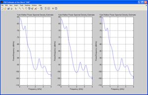
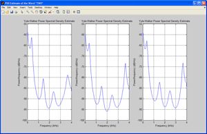
Figures 1a and 1b plot the PSD estimate of three different utterances of the words ‘one’ and ‘two’. We can see that the peaks in the PSD remain consistent for a particular digit but differ between digits. This means that we can derive the acoustic models in our system from spectral features.


From the linear predictive filter coefficients, we can obtain several feature vectors using Signal Processing Toolbox functions, including reflection coefficients, log area ratio parameters, and line spectral frequencies.
One set of spectral features commonly used in speech applications because of its robustness is Mel Frequency Cepstral Coefficients (MFCCs). MFCCs give a measure of the energy within overlapping frequency bins of a spectrum with a warped (Mel) frequency scale1.
Since speech can be considered to be short-term stationary, MFCC feature vectors are calculated for each frame of detected speech. Using many utterances of a digit and combining all the feature vectors, we can estimate a multidimensional probability density function (PDF) of the vectors for a specific digit. Repeating this process for each digit, we obtain the acoustic model for each digit.
During the testing stage, we extract the MFCC vectors from the test speech and use a probabilistic measure to determine the source digit with maximum likelihood. The challenge then becomes to select an appropriate PDF to represent the MFCC feature vector distributions.
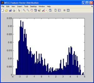
Figure 2a shows the distribution of the first dimension of MFCC feature vectors extracted from the training data for the digit ‘one’.

We could use dfittool in company/newsletters/articles/developing-an-isolated-word-recognition-system-in-matlab.html™ to fit a PDF, but the distribution looks quite arbitrary, and standard distributions do not provide a good fit. One solution is to fit a Gaussian mixture model (GMM), a sum of weighted Gaussians (Figure 2b).

The complete Gaussian mixture density is parameterized by the mixture weights, mean vectors, and covariance matrices from all component densities. For isolated digit recognition, each digit is represented by the parameters of its GMM.
To estimate the parameters of a GMM for a set of MFCC feature vectors extracted from training speech, we use an iterative expectation-maximization (EM) algorithm to obtain a maximum likelihood (ML) estimate. Given some MFCC training data in the variable MFCCtraindata, we use the Statistics and Machine Learning Toolbox gmdistribution function to estimate the GMM parameters. This function is all that is required to perform the iterative EM calculations.
  %Number of Gaussian component densities
  M = 8;
  model = gmdistribution.fit(MFCCtraindata,M);
Selecting a Classification Algorithm
After estimating a GMM for each digit, we have a dictionary for use at the testing stage. Given some test speech, we again extract the MFCC feature vectors from each frame of the detected word. The objective is to find the digit model with the maximum a posteriori probability for the set of test feature vectors, which reduces to maximizing a log-likelihood value. Given a digit model gmmmodel and some test feature vectors testdata, the log-likelihood value is easily computed using the posterior function in Statistics and Machine Learning Toolbox:
[P, log _ like] =
posterior(gmmmodel,testdata);
We repeat this calculation using each digit’s model. The test speech is classified as the digit with the GMM that produces the maximum log-likelihood value.
Building the User Interface
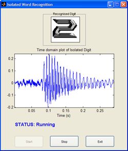
After developing the isolated digit recognition system in an offline environment with prerecorded speech, we migrate the system to operate on streaming speech from a microphone input.We use MATLAB GUIDE tools to create an interface that displays the time domain plot of each detected word as well as the classified digit (Figure 3).

Extending the Application
The algorithm described in this article can be extended to recognize isolated words instead of digits, or to recognize words from several speakers by developing a speaker-independent system.
If the goal is to implement the speech recognition algorithm in hardware, we could use MATLAB and related products to simulate fixed-point effects, automatically generate embedded C code, and verify the generated code.
Published 2010 - 91805v00