Modeling Complex Mechanical Structures with SimMechanics
By Tom Egel, MathWorks
Modeling physical components or systems in Simulink® typically involves a tradeoff between simulation speed and model fidelity or complexity: the higher the fidelity of the model, the greater the effort needed to create it. When modeling 3D mechanical structures, the task is further complicated by the need to formulate complex equations to represent the desired motion. CAD tools can sometimes be used to export models to Simulink or SimMechanics™, but this approach usually requires additional modeling resources or CAD tool expertise.
Using a wind turbine blade as an example, this article describes a semi-automated way to create complex 3D mechanical structures using MATLAB and the General Extrusion shape in SimMechanics.
Creating a Basic Model
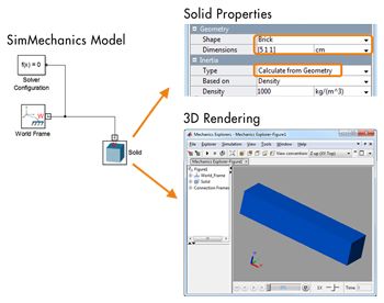
We can create a good initial model of the blade by using the default shapes in SimMechanics. The SimMechanics library contains bodies to represent the inertia, coordinate transforms to define the location in 3D space, and joints to constrain the motion of the objects within that space. Default definitions for common shapes such as sphere, cylinder, and brick automatically calculate the inertia tensor based on the dimensions you specify (Figure 1).
Specifying Complex Shapes
Using the General Extrusion shape in SimMechanics we can specify a more complex shape while still allowing SimMechanics to automatically calculate the inertia.
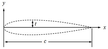
We begin by providing the outline of the wind turbine blade, using coordinate points or an equation along with the desired length to extrude the shape. We use the NACA_0015 standard1, a symmetrical airfoil shape described in the equation:
\[y_t=\frac{t}{0.2}c\left[0.2969\sqrt{\frac{x}{c}}-0.1260\left(\frac{x}{c}\right)-0.3516\left(\frac{x}{c}\right)^2+0.2843\left(\frac{x}{c}\right)^3-0.1015\left(\frac{x}{c}\right)^4\right]\]
where
\(c\) is the chord length,
\(x\) is the position along the chord from \(0\) to \(c\),
\(y\) is the half thickness at a given value of \(x\) (centerline to surface),
and \(t\) is the maximum thickness as a fraction of the chord.
Figure 2 shows the resulting shape.
To use the General Extrusion shape in SimMechanics, we must first convert the equation into a MATLAB function. The code is as follows:

Running this function from the MATLAB command line results in an array containing the points that will create the desired shape:
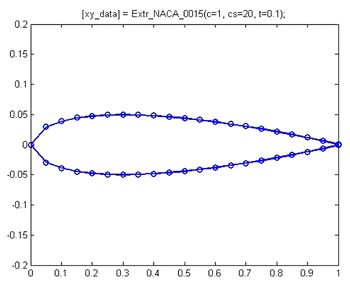
>> xy_data = Extr_NACA_0015(1,20,0.1)
We can now plot the shape in MATLAB (Figure 3).
>> plot(xy_data(:,1),xy_data(:,2),'b-o','LineWidth',1.5);
Building a Structural Model
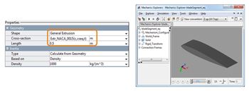
We call the MATLAB Extr_NACA_0015 function from the General Extrusion option in SimMechanics (Figure 4). The blade is represented in SimMechanics as a Solid block. Within the SimMechanics model, the Solid block calls the MATLAB Extr_NACA_0015 function, which creates the points to form the outline of the blade.
The length property specifies how long to extrude the shape. Because the Solid block is a rigid body, extruding the airfoil shape for the entire length of the blade would result in a rigid blade. To model a flexible blade, we break it into multiple segments and insert joints with stiffness and damping properties between each segment (Figure 5).
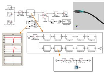
We use the test bench shown in Figure 5 to validate the model performance against measured data. During simulation we apply a known force to the tip of the blade and measure the amount of deflection along the \(x\), \(y\), and \(z\) axes. (We could use automated parameter optimization tools to tune a set of parameters to match measured test data; this is an important step in the modeling process, but beyond the scope of this article.)
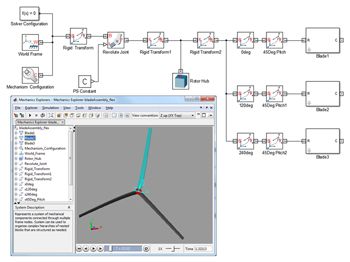
Once we have modeled and validated a single blade assembly, it is easy to connect additional assemblies to a hub to model a wind turbine blade assembly (Figure 6). We use the rigid transform blocks to position the three blades around the hub 120 degrees apart and at a fixed pitch angle of 45 degrees.
Extending This Approach
This article described the process of creating a mechanical structure using the General Extrusion shape in SimMechanics. This technique uses a set of data points to outline an arbitrary shape that can be extruded to a desired length. The data points can be entered manually or created using an equation in the form of a MATLAB function. During simulation the resulting geometry is created and the moment of inertia is automatically calculated from the shape and material properties.
We can apply the method described here to flexible bodies by partitioning the structure into multiple segments. Segments are connected by joints with spring and damping properties to model the structural stiffness. Using this modular modeling approach we can easily reuse the assembly, positioning it as desired by performing coordinate transformations. We could use MATLAB to further speed up the modeling process by automatically constructing the blade assembly based on input we provide (such as blade length, number of blades, number of segments, and material properties). Ultimately, this blade assembly could be used in a system simulation with electrical or hydraulic actuators to control the hub speed and blade pitch.
1The equations to precisely describe common wing profiles are provided by the National Advisory Committee for Aeronautics (NACA; https://en.wikipedia.org/wiki/NACA_airfoil).
Published 2013 - 92150v00