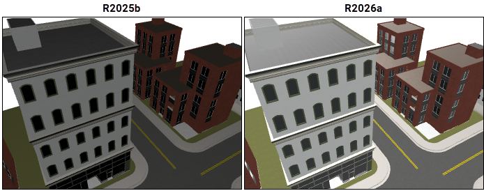
When you read a scene model from a GL Transmission Format (glTF™) file into Site Viewer by using the siteviewer function, the model has a brighter appearance. This image
compares a scene model in Site Viewer in R2025b and R2026a.
Optimize large antennas and arrays using the TR-SADEA algorithm in the Antenna Designer and Antenna Array
Designer apps. To select the TR-SADEA as your optimizer, select
TR-SADEA option under the
Optimizer drop down menu in the
OPTIMIZER tab.
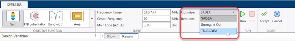
You can use the TR-SADEA algorithm to optimize antennas and arrays for various objective functions within the associated constraints. To use this feature, you need a Statistics and Machine Learning Toolbox™ license.
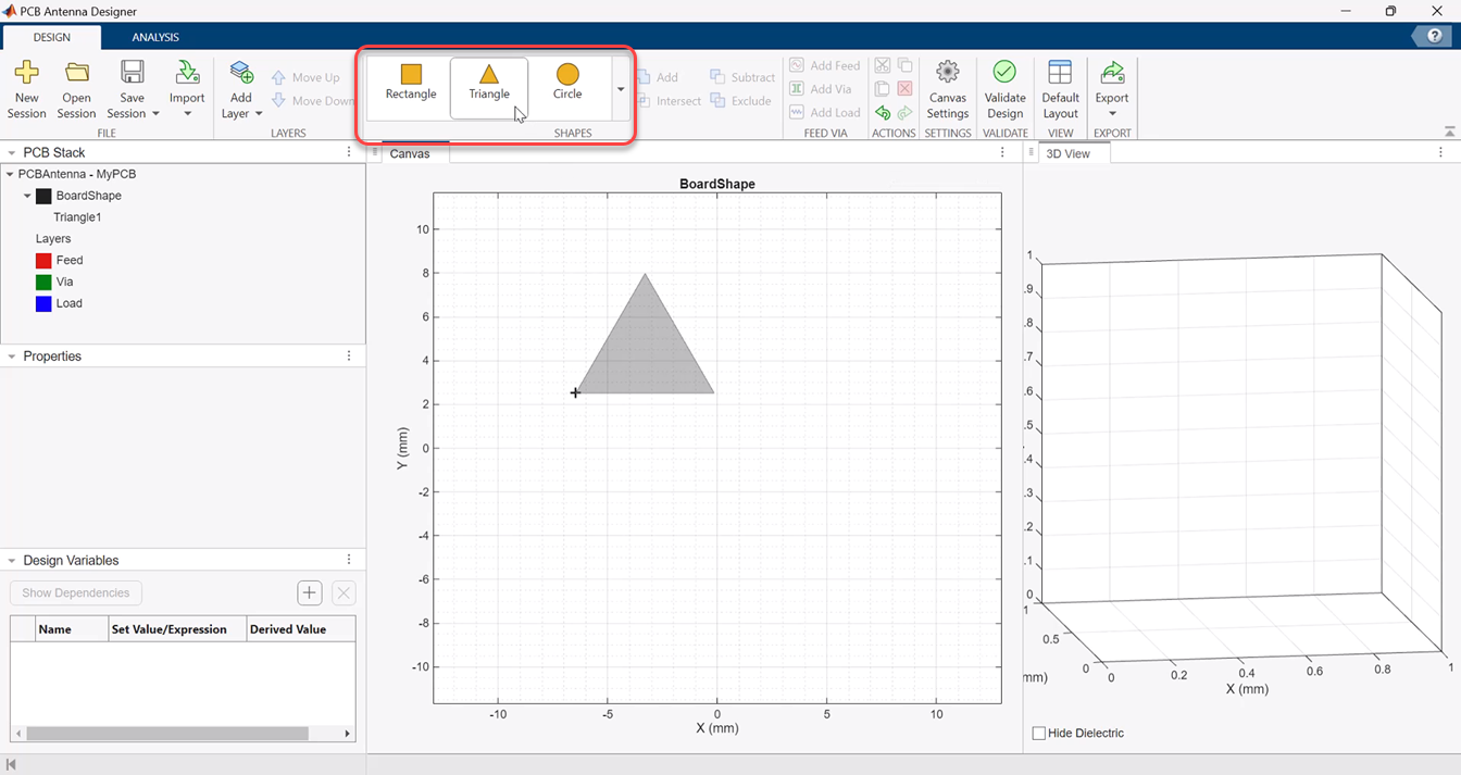
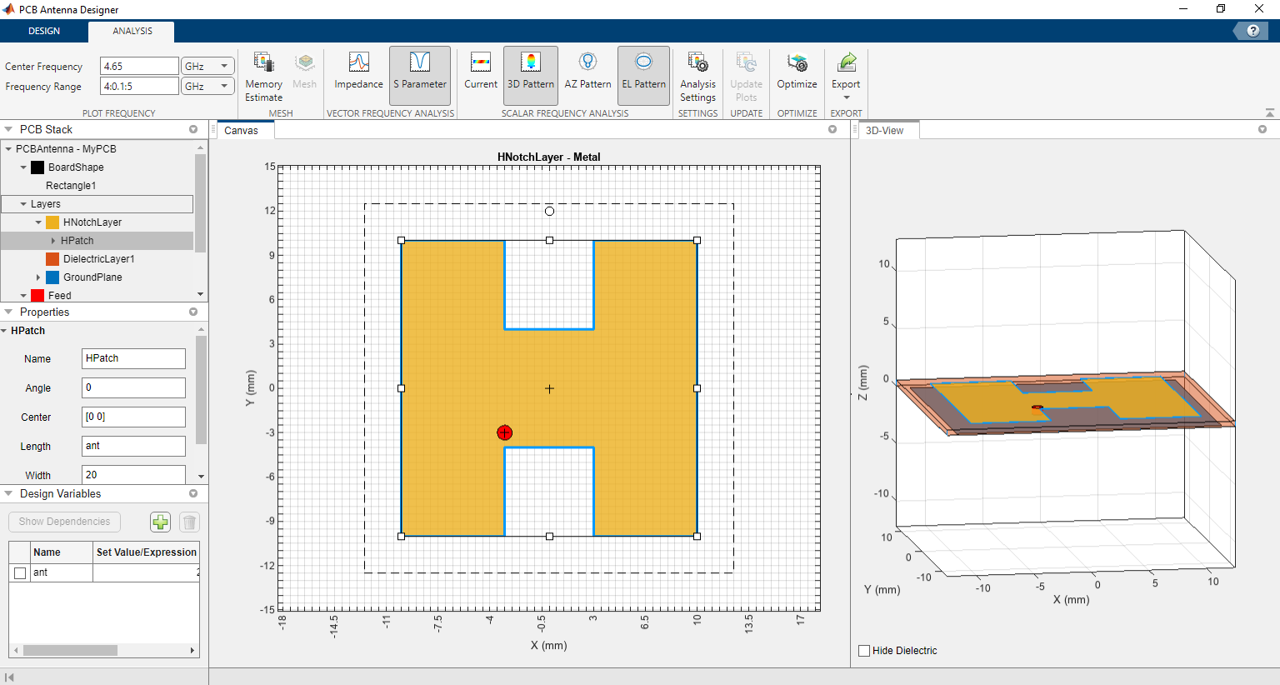
The shapes catalog in the PCB Antenna Designer app now has a triangular shape.
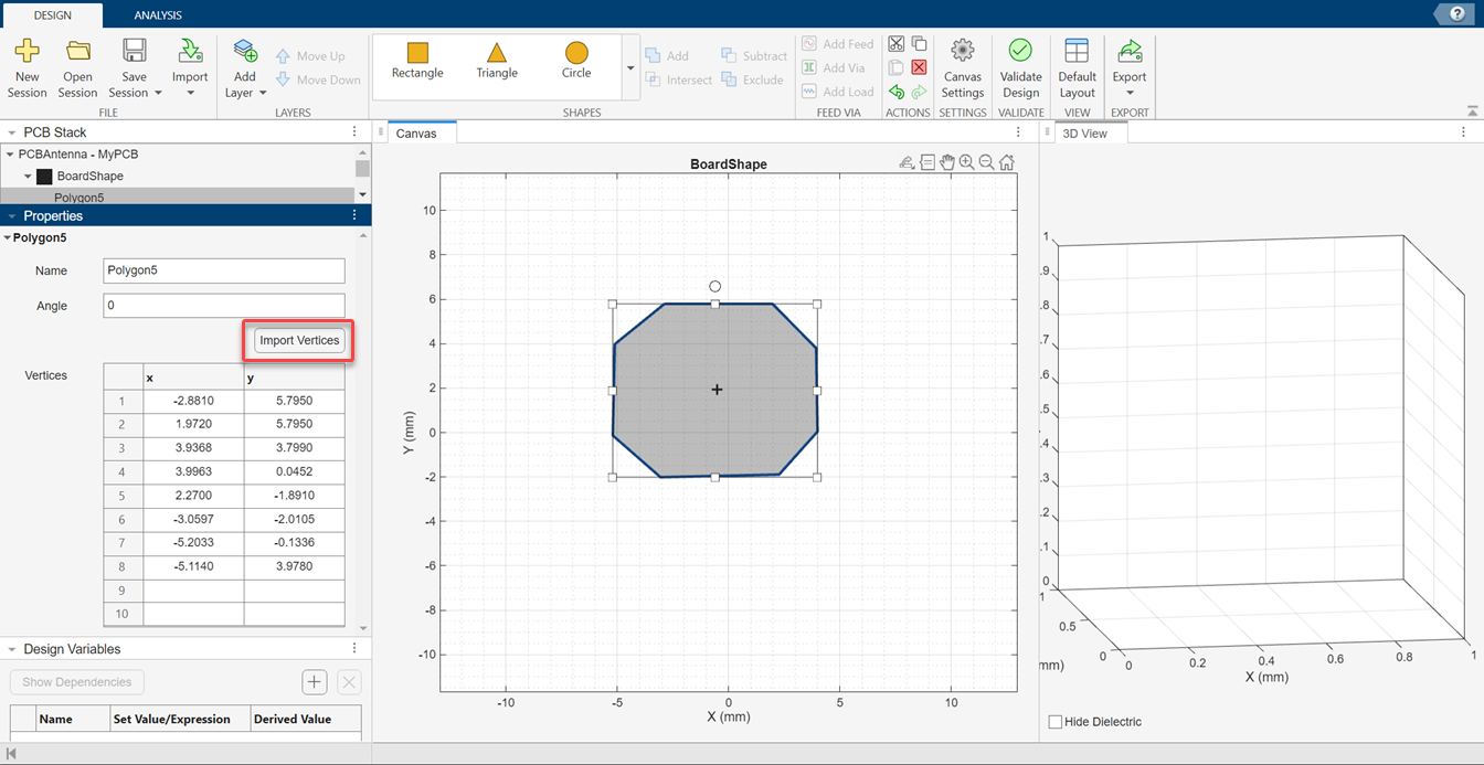
The PCB Antenna Designer app now lets you import polygon vertices data from a workspace variable.
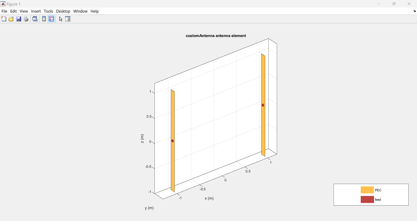
The createFeed function of customAntenna now enables you to interactively add multiple
single-edge and multi-edge feed points to the custom antenna or array.
Provide customAntenna object as the only input argument to the
createFeed function to open an interactive window. Click
the feed edges to select them.
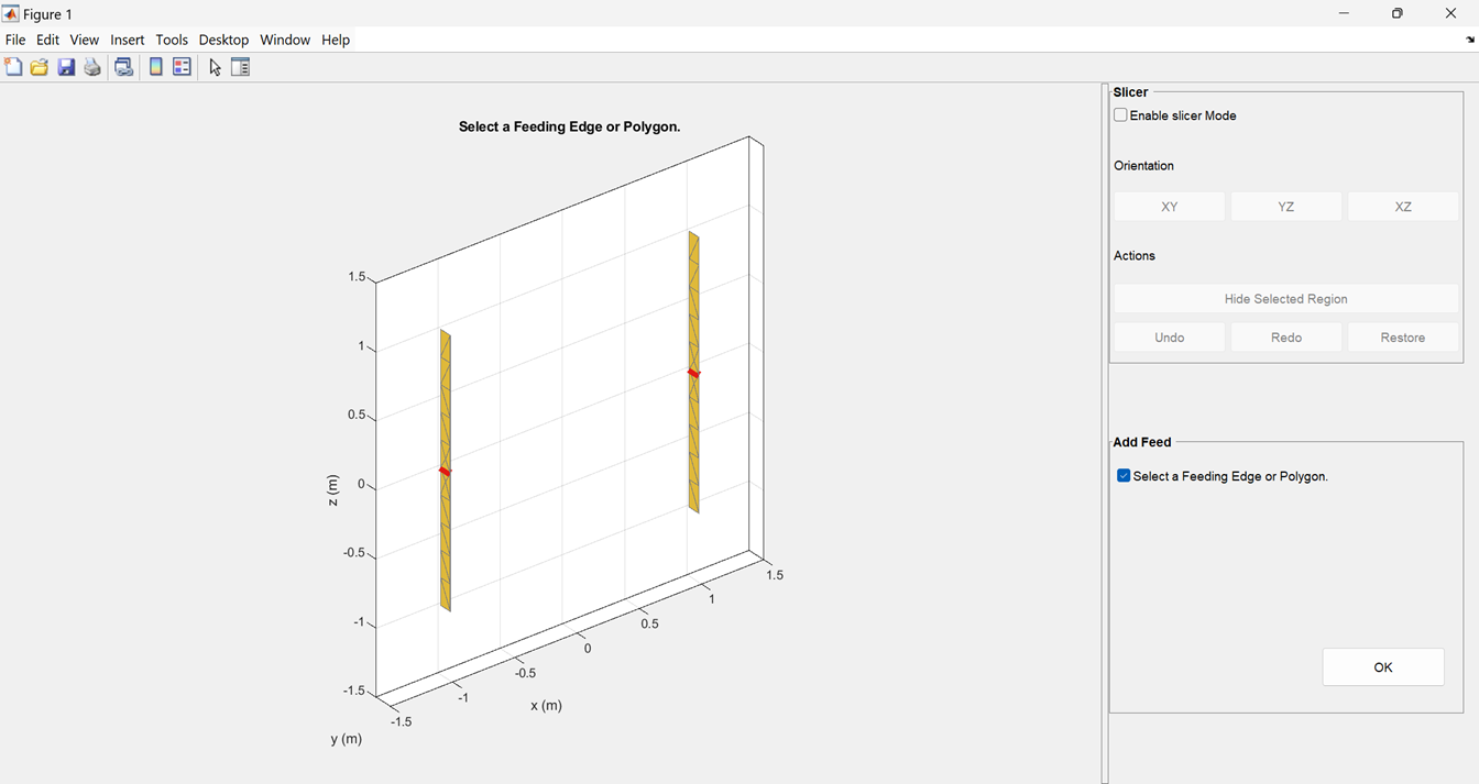
After selecting the edges, click OK to create feed points.
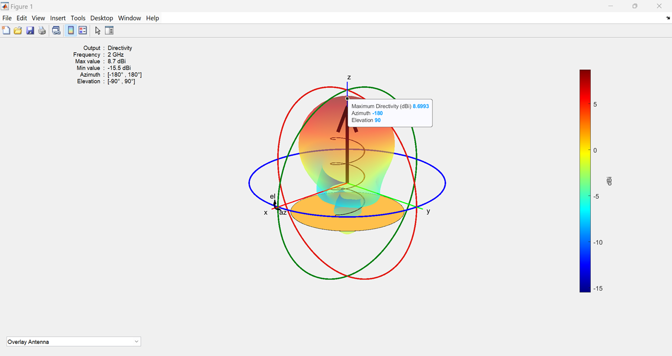
Use the new peakRadiation function to calculate and plot the maximum radiation
of an antenna or array. This function calculates and plots maximum gain:
For the antennas with a dielectric substrate other than air.
For the antennas with conductor metal other than PEC.
This function calculates and plots maximum directivity:
For the antennas without a dielectric substrate or with the air substrate.
For the antennas with PEC conductor.
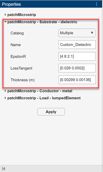
You can now use the Antenna Designer and Antenna Array Designer apps to design an antenna or array with a dielectric substrate. You can choose a predefined dielectric material from a drop-down list or you can specify your own material by changing the default dielectric properties. You can also specify multiple dielectric materials by providing vector inputs to the dielectric properties.
This image shows the Antenna Designer toolstrip with the option to select the dielectric substrate.

This image shows the Antenna Array Designer toolstrip with the option to select the dielectric substrate.
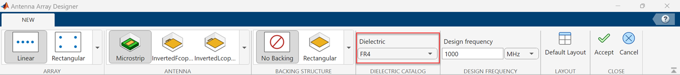
To create a custom dielectric, change the default substrate properties.

To specify multiple dielectrics, select Multiple in the
Catalog list and specify values as a vector.
Use custom geometric constraints defined by linear equalities and inequalities and nonlinear inequalities for antenna or array optimization. You can define the custom geometric constraints in the Geometric Constraints panel of the Optimizer tab using the coefficients of linear inequalities (A, b), equalities (Aeq, beq), and nonlinear inequalities (nlcon, nrlv).
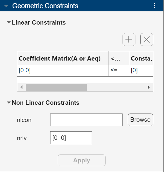
For additional information on linear and nonlinear equalities and nonlinear
inequalities, see the fmincon (Optimization Toolbox) function documentation.
Use the new patternSystem function to simultaneously visualize the 3-D radiation
patterns of multiple antennas mounted on a platform.

You can now generate a mesh manually by setting the mesh parameters such as maximum edge length, minimum edge length, and growth rate in the Antenna Designer and Antenna Array Designer. You can set these parameters by clicking the Analysis Settings button in the Settings section and changing the mesh mode to manual.

You can now view the memory required by the Antenna Designer and Antenna Array Designer apps to solve an antenna or array mesh. You can view the estimated memory by clicking the Memory Estimate button in the Mesh section of the app toolstrip. You can reduce the memory requirement by clicking the Analysis Settings button in the Settings section, changing the mesh mode from automatic to manual and adjusting the mesh parameter values.

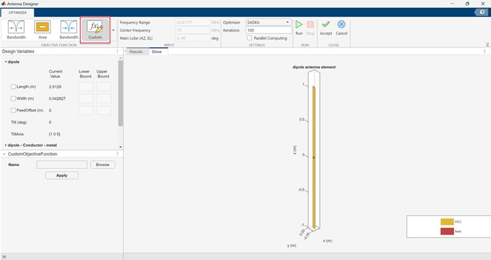
You can now specify a custom objective function to define antenna or array
optimization objectives in the optimize function or the Antenna Designer, Antenna Array
Designer and PCB Antenna
Designer apps.
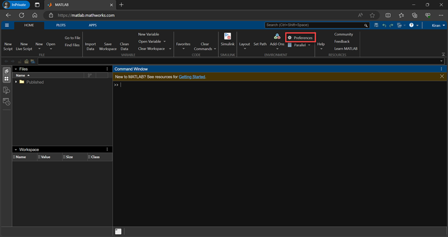
Antenna Toolbox is now available in the MATLAB Online™ environment. For more information, see MATLAB Online (MATLAB Online Server).
Antenna Toolbox in MATLAB Online supports dark theme visualization. To select the
dark theme, on the Home tab, in the
Environment section, click ![]() Preferences. Select MATLAB > Appearance and set the Theme to
Dark.
Preferences. Select MATLAB > Appearance and set the Theme to
Dark.
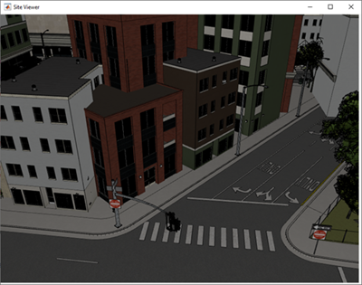
Import glTF files
Read a scene model from a GL Transmission Format (glTF) file with the
.gltf or .glb extension into Site Viewer
by using the siteviewer function. Specify the name of the model by using the
SceneModel name-value argument. Site Viewer displays the
model using the colors and textures stored in the file.
This figure shows a Site Viewer window with a scene model read from a glTF file. The file was created using RoadRunner.
Display buildings using colors from OpenStreetMap files
When you read buildings data from an OpenStreetMap file into Site Viewer, Site Viewer displays the buildings using the colors stored in the file.
Import customized buildings data
Import customized buildings data into Site Viewer by using geospatial tables that contain buildings data. This capability requires Mapping Toolbox™.
Read buildings from an OpenStreetMap file with the
.osmextension into a geospatial table by using thereadgeotable(Mapping Toolbox) function. Specify theLayername-value argument as"buildings"or"buildingparts".Customize the buildings by editing the geospatial table. For example, you can change the footprints, heights, colors, and materials of the buildings.
Import the geospatial table into Site Viewer by using the
siteviewerfunction. Specify the geospatial table using theBuildingsname-value argument. Site Viewer displays the buildings using the colors stored in the table.
For an example that shows how to import customized buildings data into Site Viewer, see Customize Buildings for Ray Tracing Analysis.
Perform ray tracing analysis using multiple materials in the same scene
When you perform ray tracing analysis on a scene created from a glTF file, an OpenStreetMap file, or a geospatial table, the ray tracing
analysis uses the materials specified by the file or table. Functions that can
perform ray tracing analysis include raytrace, coverage, sigstrength, link, and sinr.
When you create a scene from a glTF file, an OpenStreetMap file, or a geospatial table, Site Viewer assigns materials to the
surfaces in the scene by matching the material names stored in the file or table
with the material names supported by the RayTracing propagation model object. Then, Site Viewer stores the
material names in the Materials property. When you perform ray
tracing analysis by using a function such as raytrace or
coverage, the function uses the material names stored in
the Materials property. The Materials
property is read-only.
Scale the size of scene models
You can now change the scale of scene models created from glTF files, STL files, and triangulation objects by specifying the
SceneModelScale name-value argument of the siteviewer function. By default, Site Viewer interprets scene models
using units of meters with a 1:1 scale.
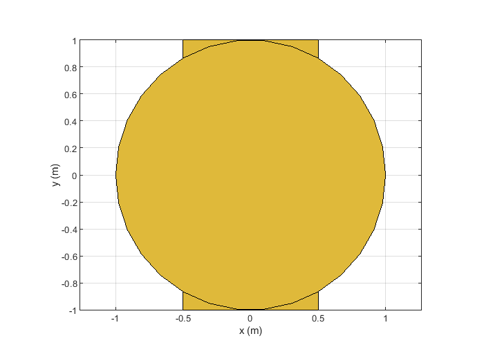
Use the hold on functionality to display multiple shapes from
the shape catalog on the same figure.
show(antenna.Rectangle)
hold on
show(antenna.Circle)
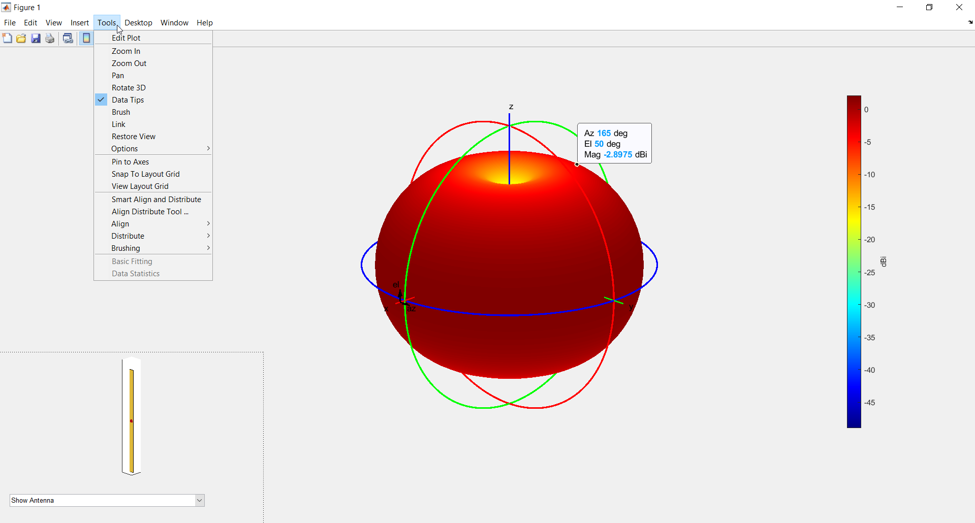
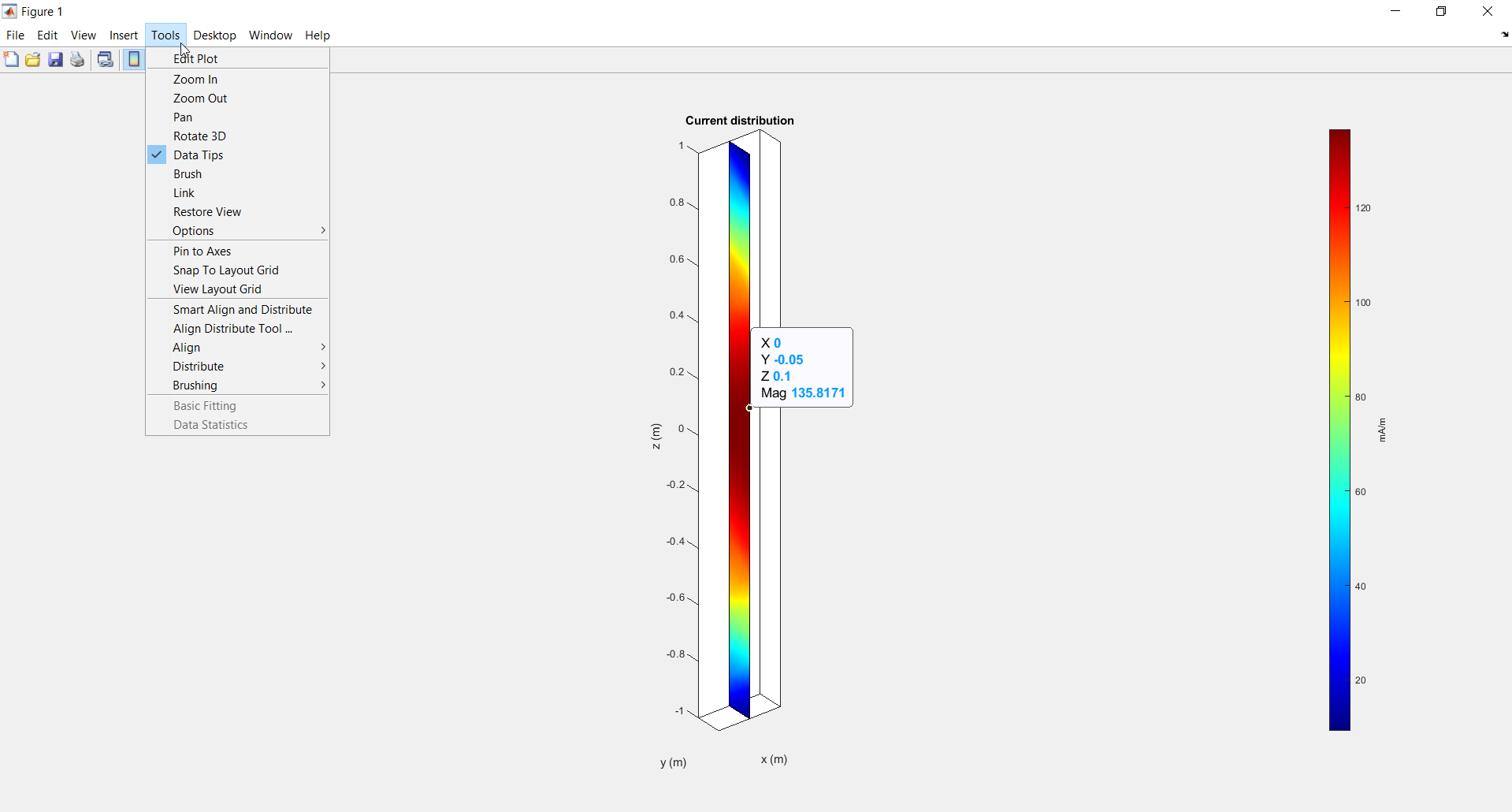
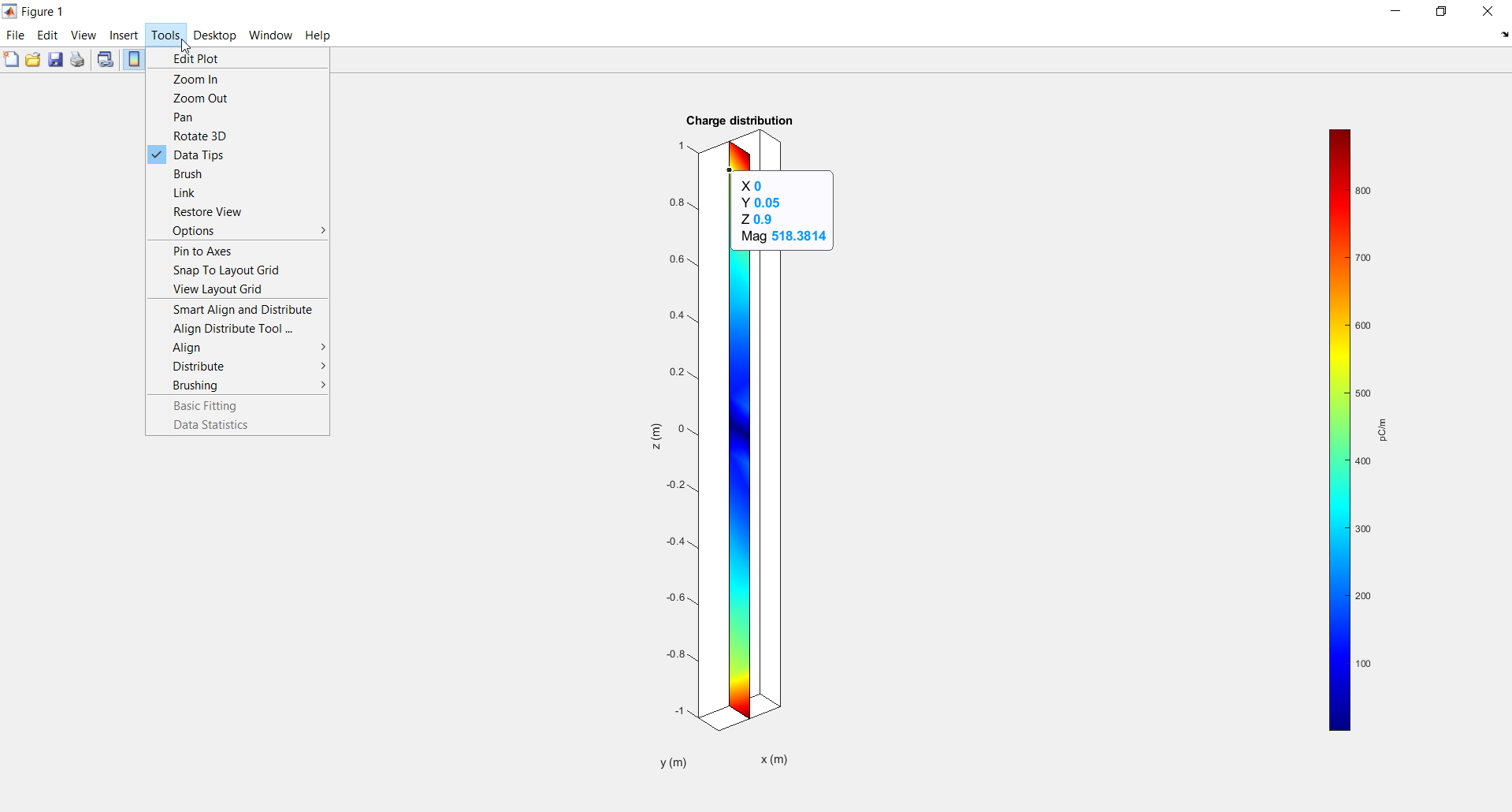
Use the Data Tip option under Tools menu
in the figure window to view the values of position and magnitude at that position
for pattern, current, and
charge plots. Data Tip on a:
Ray tracing models enable you to discard propagation paths based on path loss
thresholds. To specify the thresholds, create a RayTracing object and set its MaxAbsolutePathLoss
and MaxRelativePathLoss properties.
Specify an absolute threshold by using the
MaxAbsolutePathLossproperty. For example, you can discard paths with more than 100 decibels of path loss by specifyingMaxAbsolutePathLossas100. The default value isInf, which does not discard paths based on absolute path loss.Specify a threshold relative to the strongest propagation path by using the
MaxRelativePathLossproperty. The default value is40, which discards paths that are more than 40 decibels weaker than the strongest path.
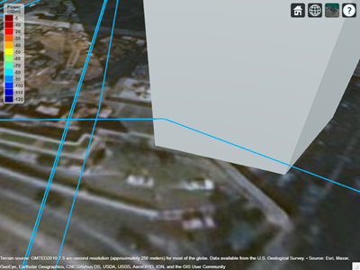
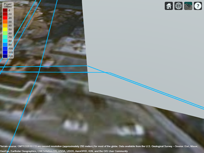
This capability can simplify visualizations in Site Viewer. For
example, these two images visualize propagation paths for the same transmitter and
receiver. The image on the left uses a model where
MaxRelativePathLoss is Inf, and the
image on the right uses a model where MaxRelativePathLoss is
40 (the default).

The default value of the MaxRelativePathLoss property is
40. As a result, code from previous releases that does
not specify a MaxRelativePathLoss value can be affected in
these ways:
The
raytracefunction can return fewercomm.Rayobjects in R2023a compared to previous releases.The
sigstrength,coverage,sinr, andlinkfunctions can return different values in R2023a compared to previous releases.The
pathlossfunction can return different path loss values in R2023a compared to previous releases.
To avoid discarding propagation paths, set the
MaxRelativePathLoss property of the ray tracing object
to Inf.
You can now optimize PCB antenna designs using the SADEA and surrogate optimization methods in the PCB Antenna Designer app. Create design variables to enable the optimization process. Optimize your designs for bandwidth, gain, front-to-back-lobe ratio, and area.
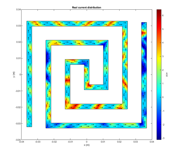
The current function now takes these new name-value arguments
Type-- Choose between the absolute, real, or imaginary values of the current vector to plot the current distribution.Direction-- Plot the direction of the current flow overlaid on the distribution plot.
When you find propagation paths by using the raytrace function and the shooting and bouncing rays (SBR) method,
MATLAB corrects the results so that the geometric accuracy of each path is
exact, using single-precision floating-point computations. In previous releases, the
paths have approximate geometric accuracy.
For example, this code finds propagation paths between a transmitter and receiver
by using the default SBR method and returns the paths as comm.Ray
objects. In R2022b, the raytrace function finds seven
propagation paths. In earlier releases, the function approximates eight propagation
paths, one of which is a duplicate path.
viewer = siteviewer(Buildings="hongkong.osm");

tx = txsite(Latitude=22.2789,Longitude=114.1625,AntennaHeight=10, ...
   TransmitterPower=5,TransmitterFrequency=28e9);
rx = rxsite(Latitude=22.2799,Longitude=114.1617,AntennaHeight=1);

rSBR = raytrace(tx,rx)
raytrace(tx,rx)
| R2022b | R2022a |
|---|---|
rSBR =

  1×1 cell array

    {1×7 comm.Ray}
|
rSBR =

  1×1 cell array

    {1×8 comm.Ray}
|
Paths calculated using the SBR method in R2022b more closely align with paths calculated using the image method. The image method finds all possible paths with exact geometric accuracy. For example, this code uses the image method to find propagation paths between the same transmitter and receiver.
viewer = siteviewer(Buildings="hongkong.osm");

tx = txsite(Latitude=22.2789,Longitude=114.1625, ...
   AntennaHeight=10,TransmitterPower=5, ...
   TransmitterFrequency=28e9);
rx = rxsite(Latitude=22.2799,Longitude=114.1617, ...
   AntennaHeight=1);

pm = propagationModel("raytracing",Method="image",MaxNumReflections=2);

rImage = raytrace(tx,rx,pm)
rImage =

  1×1 cell array

    {1×7 comm.Ray}
In this case, the SBR method finds the same number of propagation paths as the image method. In general, the SBR method finds a subset of the paths found by the image method. When both the image and SBR methods find the same path, the points along the path are the same within a tolerance of machine precision for single-precision floating-point values.
This code compares the path losses, within a tolerance of
0.0001, calculated by the SBR and image methods.
abs([rSBR{1}.PathLoss]-[rImage{1}.PathLoss]) < 0.0001ans = 1×7 logical array 1 1 1 1 1 1 1
The path losses are the same within the specified tolerance.
The raytrace function can return different results in
R2022b compared to previous releases.
The function can return a different number of
comm.Rayobjects because it discards invalid or duplicate paths.The function can return different
comm.Rayobjects because it calculates exact paths rather than approximate paths.
These differences can also affect the path losses calculated by
the raypl and pathloss functions.