Maximize Impedance Bandwidth of Triangular Patch Antenna

This example shows how to optimize a triangular microstrip patch antenna to maximize its bandwidth such that its gain remains constant.

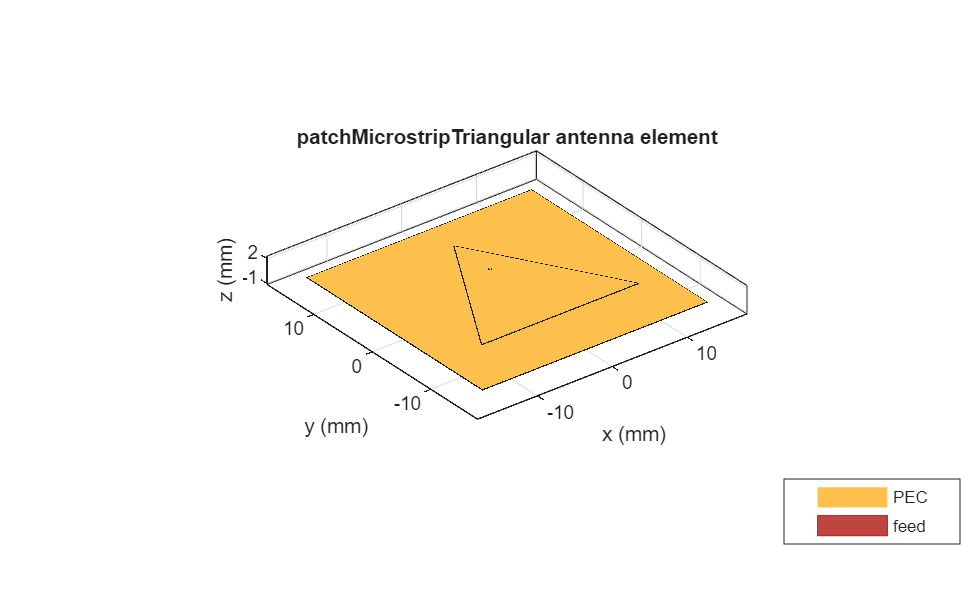
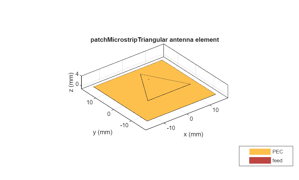
Define Antenna Geometry

Define the initial geometry of the antenna.

% Define Antenna
ant = patchMicrostripTriangular;

% Center frequency and frequency range 
fc = 10e9;
% For BW ~20%
minFreq = fc * 0.8;
maxFreq = fc * 1.2;
freqRange = linspace(minFreq, maxFreq, 35);

% Initial point
ant = design(ant, fc)

ant = 
  patchMicrostripTriangular with properties:

                 Side: 0.0210
               Height: 0.0012
            Substrate: [1×1 dielectric]
    GroundPlaneLength: 0.0300
     GroundPlaneWidth: 0.0300
    PatchCenterOffset: [0 0]
           FeedOffset: [0 0.0029]
         FeedDiameter: 3.7474e-04
            Conductor: [1×1 metal]
                 Tilt: 0
             TiltAxis: [1 0 0]
                 Load: [1×1 lumpedElement]

Use show function to view the antenna.

show(ant) 

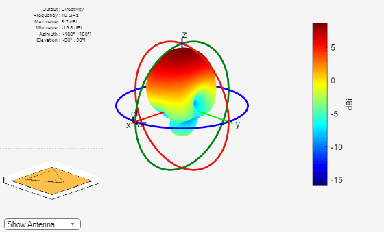
Initial Analysis

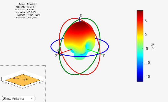
Analyze the gain of the antenna. Record the maximum gain of the antenna before optimization.

pattern(ant, fc);

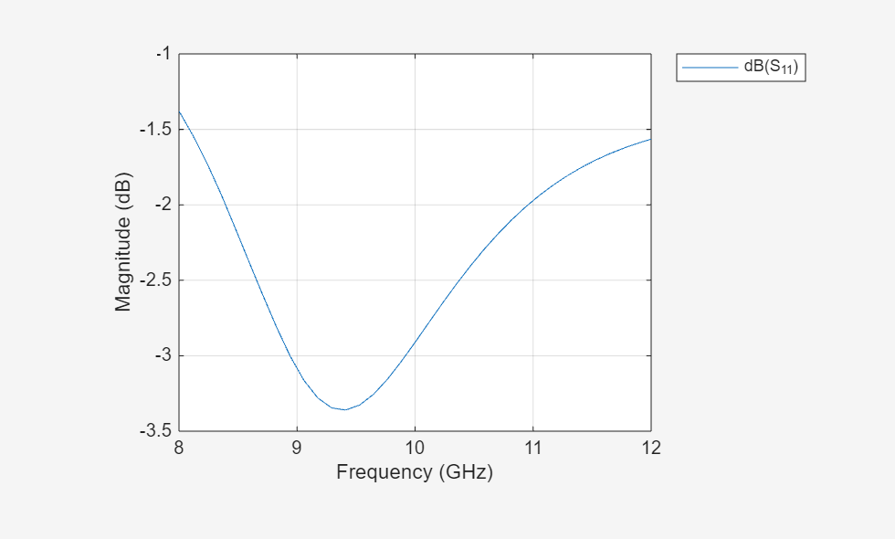
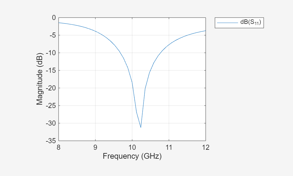
Analyze the impedance bandwidth of the antenna using S-parameters.

rfplot(sparameters(ant, freqRange));

Set Up Optimization Problem

You will need the following inputs for the optimization problem:

1. Objective Function: Choose 'maximizeBandwidth' as the objective function. The main goal of this example is maximizing the bandwidth of the antenna.

2. Design variables: Select side length, height of the triangular patch antenna, and feed offset as control variables for the objective function. The side length of the triangular patch will affect the front lobe gain. The height and the feed location will enhance the impedance bandwidth of the antenna and help improve its matching.

3. Constraints: The constraint function is gain more than 8.5 dBi.

% Design Variables
% Property Names
propNames = {'Side', 'Height', 'FeedOffset'};

% Bounds for the properties {lower bounds; upper bounds}          
bounds = {0.017 0.001 [0 0.0017]; ... % Specify the FeedOffset vector to move the feed along [x, y]
    0.023 0.004 [0.0002 0.0034]};

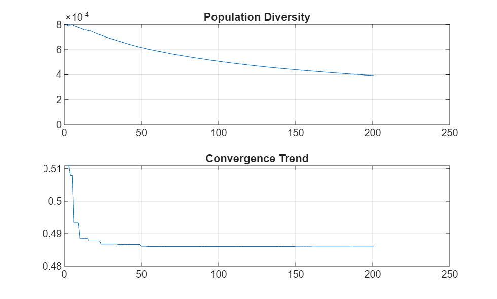
Optimization Function

To optimize the antenna, use the optimize function.

figure; % Figure to display the convergence trend
% Optimize
optAnt = optimize(ant, fc, 'maximizeBandwidth', ...
    propNames, bounds, ...
    'Constraints', {'Gain > 8.5'}, ...
    'FrequencyRange', freqRange, ...
    'UseParallel', true);

Starting parallel pool (parpool) using the 'local' profile ...
Connected to the parallel pool (number of workers: 6).

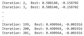
Set 'EnableLog' as true, in order to print the iteration number and best value of convergence on the command line.

Optimization Result

Compare the analysis parameters of the antenna from before and after the optimization.

optAnt

optAnt = 
  patchMicrostripTriangular with properties:

                 Side: 0.0190
               Height: 0.0029
            Substrate: [1×1 dielectric]
    GroundPlaneLength: 0.0300
     GroundPlaneWidth: 0.0300
    PatchCenterOffset: [0 0]
           FeedOffset: [2.4368e-05 0.0033]
         FeedDiameter: 3.7474e-04
            Conductor: [1×1 metal]
                 Tilt: 0
             TiltAxis: [1 0 0]
                 Load: [1×1 lumpedElement]

show(optAnt) 

pattern(optAnt, fc)

rfplot(sparameters(optAnt, freqRange))

Observe the bandwidth of the antenna after optimization.