Main Content

rnaseqde

Perform differential expression analysis on RNA-seq count data

Since R2021b

Description

example

diffTable = rnaseqde(countTable,conditionVariables1,conditionVariables2) uses the RNA-seq count data in countTable and performs differential expression analysis between the conditions (or samples) in conditionVariables1 and conditionVariables2. The rows of countTable represent genes (or features), and the columns represent the conditions. The function first divides each condition by a library size factor to normalize the count prior to performing the hypothesis test. This size factor is equal to the median ratio of each feature over the geometric mean of the feature in all conditions. The function uses an exact test to determine the differences between two groups of counts that are each assumed to follow a negative binomial distribution [1].

example

diffTable = rnaseqde(___,Name=Value) specifies additional options using one or more name-value arguments.

Examples

collapse all

Use RNA-seq count data that consists of two biological replicates of the control (untreated) samples and two biological replicates of the knock-down (treated) samples [6]. Load the table with read counts for genes.

load("pasilla_count_noMM.mat","geneCountTable")

Display the first few rows of the table.

head(geneCountTable,10)
         ID          Reference    untreated3    untreated4    treated2    treated3
    _____________    _________    __________    __________    ________    ________

    "FBgn0000003"      "3R"             0             1            1           2  
    "FBgn0000008"      "2R"           142           117          138         132  
    "FBgn0000014"      "3R"            20            12           10          19  
    "FBgn0000015"      "3R"             2             4            0           1  
    "FBgn0000017"      "3L"          6591          5127         4809        6027  
    "FBgn0000018"      "2L"           469           530          492         574  
    "FBgn0000024"      "3R"             5             6           10           8  
    "FBgn0000028"      "X"              0             0            2           1  
    "FBgn0000032"      "3R"          1160          1143         1138        1415  
    "FBgn0000036"      "3R"             0             0            0           1  

Perform the differential analysis of the control and treated samples using the read count data for genes. Specify both replicates for each condition. The input geneCountTable has an ID column. Optionally, you can append this column to the output table by using IDColumns.

diffTable = rnaseqde(geneCountTable,["untreated3", "untreated4"],...
                     ["treated2", "treated3"],IDColumns="ID");
head(diffTable,5)
         ID           Mean1      Mean2     Log2FoldChange     PValue      AdjustedPValue
    _____________    _______    _______    ______________    _________    ______________

    "FBgn0000003"    0.51415     1.3808         1.4253               1              1   
    "FBgn0000008"      135.9     129.48      -0.069799         0.67298        0.89231   
    "FBgn0000014"     16.838     13.384       -0.33119          0.6421        0.87234   
    "FBgn0000015"     3.1234    0.42413        -2.8806         0.22776        0.57215   
    "FBgn0000017"     6151.8     5117.4       -0.26559       0.0014429       0.014207   

Look at the difference in gene expression between two conditions by displaying the log2 fold change for each gene.

figure
scatter(log2(mean([diffTable.Mean1,diffTable.Mean2], 2)),diffTable.Log2FoldChange,3,diffTable.AdjustedPValue,'o')
colormap(flipud(cool(256)))
colorbar;
ylabel("log2(Fold change)")
xlabel("log2(Mean of normalized counts)")
title("Fold change by FDR")

You can also annotate the values in the plot with the corresponding gene names, interactively select genes, and export gene lists to the workspace.

warnSettings = warning('off','bioinfo:mairplot:ZeroValues');
mairplot(diffTable.Mean2,diffTable.Mean1,Labels=geneCountTable.ID,Type="MA");
set(get(gca,"Xlabel"),"String","mean of normalized counts")
set(get(gca,"Ylabel"),"String","log2(fold change)")

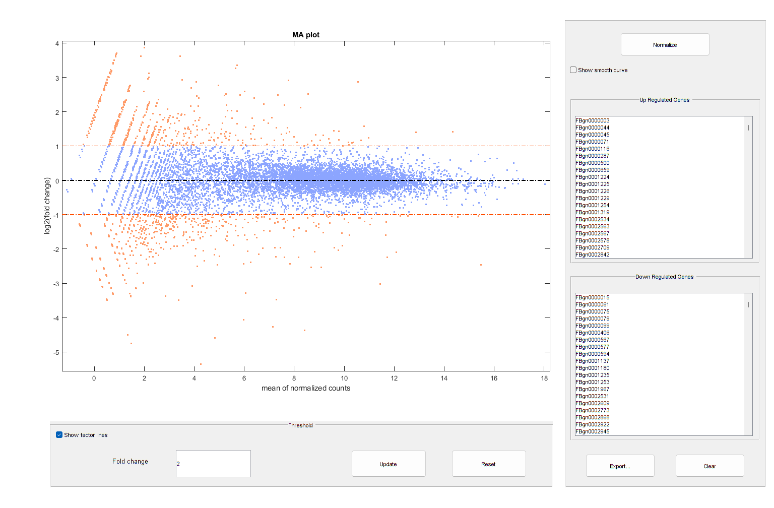
warning(warnSettings);

Input Arguments

collapse all

RNA-seq count data, specified as a table. It contains counts of genomic features for all replicates of each condition.

Data Types: table

Table variables for the first condition, specified as a cell array of character vectors, string vector, or numeric vector. You can specify a list of table variable names of the corresponding columns in countTable or a numeric vector containing the indices of the columns.

Data Types: cell | double | string

Table variables for the second condition, specified as a cell array of character vectors, string vector, or numeric vector. You can specify a list of table variable names of the corresponding columns in countTable or a numeric vector containing the indices of the columns.

Data Types: cell | double | string

Name-Value Arguments

Specify optional pairs of arguments as Name1=Value1,...,NameN=ValueN, where Name is the argument name and Value is the corresponding value. Name-value arguments must appear after other arguments, but the order of the pairs does not matter.

Before R2021a, use commas to separate each name and value, and enclose Name in quotes.

Example: dt = rnaseqde(ct,[1 3],[4 6],FDRMethod="storey") specifies to use the Storey procedure as the false discovery rate method.

Linkage type between the variance and mean, specified as a character vector or string. This table summarizes the available linkage options.

Linkage optionDescriptionWhen to use
"local"The variance is the sum of the shot noise term (mean) and a locally regressed nonparametric smooth function of the mean as described in [1]. This option is the default. Use this option if your data is overdispersed and has more than 1000 rows (genes).
"constant"The variance is the sum of the shot noise term (mean) and a constant multiplied by the squared mean as described in [2]. This method uses all the rows in the data to estimate the constant. Use this option if your data is overdispersed and has less than 1000 rows.
"identity"The variance is equal to the mean as described in [3]. Counts are therefore modeled by the Poisson distribution individually for each row of the conditions. Use this option if your data has few genes and the regression between the variance and mean is not possible because of a very small number of samples or replicates. This option is not recommended for overdispersed data.

False discovery rate method to adjust p-values, specified as "bh" or "storey". By default, the function uses "bh", which is the linear step-up procedure introduced by Benjamini and Hochberg [4]. The "storey" method adjusts p-values using the procedure introduced by Storey [5].

Columns from the input countTable to append to the output diffTable, specified as a character vector, string, string vector, cell array of character vectors, or numeric vector. You can specify the column names or a numeric vector containing the indices of the columns in countTable. The function appends the columns to the left side of the output table.

Data Types: double | char | string | cell

Output Arguments

collapse all

Differential expression analysis results, returned as a table with these columns:

  • Mean1 — Mean normalized counts for the samples specified in conditionVariables1

  • Mean2 — Mean normalized counts for the samples specified in conditionVariables2

  • Log2FoldChange — Log2 ratio of Mean2 over Mean1

  • PValue — P-value output from the hypothesis test

  • AdjustedPValue — Adjusted p-value, calculated using the method specified in 'FDRMethod'

References

[1] Anders, Simon, and Wolfgang Huber. “Differential Expression Analysis for Sequence Count Data.” Genome Biology 11, no. 10 (October 2010): R106. https://doi.org/10.1186/gb-2010-11-10-r106.

[2] Robinson, Mark D., and Gordon K. Smyth. “Small-Sample Estimation of Negative Binomial Dispersion, with Applications to SAGE Data.” Biostatistics 9, no. 2 (July 11, 2007): 321–32.

[3] Marioni, J. C., C. E. Mason, S. M. Mane, M. Stephens, and Y. Gilad. “RNA-Seq: An Assessment of Technical Reproducibility and Comparison with Gene Expression Arrays.” Genome Research 18, no. 9 (July 30, 2008): 1509–17.

[4] Benjamini, Y., and Hochberg, Y. 1995. Controlling the false discovery rate: A practical and powerful approach to multiple testing. J. Royal Stat. Soc. 57:289–300.

[5] Storey, John D. “A Direct Approach to False Discovery Rates.” Journal of the Royal Statistical Society: Series B (Statistical Methodology) 64, no. 3 (August 2002): 479–98.

[6] Brooks, A. N., L. Yang, M. O. Duff, K. D. Hansen, J. W. Park, S. Dudoit, S. E. Brenner, and B. R. Graveley. “Conservation of an RNA Regulatory Map between Drosophila and Mammals.” Genome Research 21, no. 2 (February 1, 2011): 193–202.

Version History

Introduced in R2021b