eyediagram
Generate eye diagram
Syntax
Description
eyediagram(
specifies plot attributes for the eye diagram.x,n,period,offset,plotstring)
h = eyediagram(___)
Examples
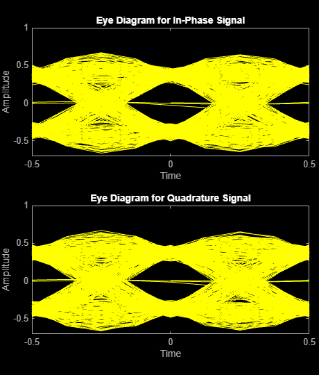
Generate an eyediagram of a filtered QPSK signal.
Generate random symbols. Apply QPSK modulation to get a modulated signal.
data = randi([0 3],1000,1);
modSig = pskmod(data,4,pi/4);
Specify the number of output samples per symbol parameter. Create a transmit filter object, txfilter.
sps=4;
txfilter = comm.RaisedCosineTransmitFilter('OutputSamplesPerSymbol',sps);
Filter the modulated signal modSig.
txSig = txfilter(modSig);
Display the eye diagram.
eyediagram(txSig,2*sps)
Input Arguments
Output Arguments
Version History
Introduced before R2006a