Visualize RF Impairments
Apply various RF impairments to a QAM signal. Observe the effects by using constellation diagrams, time-varying error vector magnitude (EVM) plots, and spectrum plots. Estimate the equivalent signal-to-noise ratio (SNR) by using the modulation error rate (MER) measurement.
Initialization
Set the sample rate, modulation order, and SNR. Calculate the reference constellation points. Generate a 16-QAM signal.
fs = 1000;
M = 16;
snrdB = 30;
refConst = qammod(0:M-1,M,UnitAveragePower=true);
data = randi([0 M-1],1000,1);
modSig = qammod(data,M,UnitAveragePower=true);
Create constellation diagram and time scope objects to visualize the impairment effects.
constDiagram = comm.ConstellationDiagram( ...
    ReferenceConstellation=refConst);
timeScope = timescope( ...
    YLimits=[0 40], ...
    SampleRate=fs, ...
    TimeSpanSource="property", ...
    TimeSpan=1, ...
    ShowGrid=true, ...
    YLabel="EVM (%)");
Amplifier Distortion
Memoryless nonlinear impairments distort the amplitude and phase of the input signal. The amplitude distortion is amplitude-to-amplitude modulation (AM-AM) and the phase distortion is amplitude-to-phase modulation (AM-PM). The memoryless nonlinearity System object™ models AM-AM and AM-PM distortion that result from amplifier gain compression and AM-PM conversion, respectively.
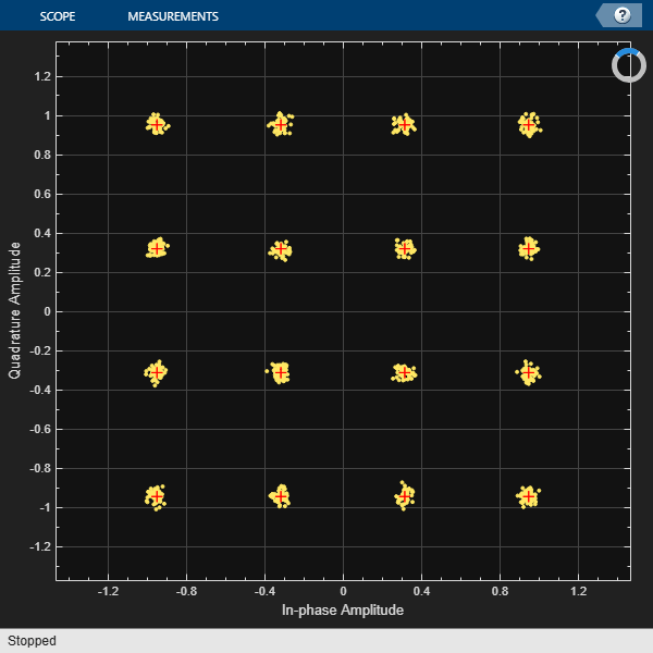
Add amplifier gain compression with no AM-PM conversion impairment by using a memoryless nonlinearity object. Amplifier gain compression is a nonlinear impairment that distorts symbols more as the distance from the origin increases.
mnlamp= comm.MemorylessNonlinearity( ...
    Method="Modified Rapp model", ...
    Smoothness=1.4);
Pass the modulated signal through the nonlinear amplifier, and then plot constellation diagram. The amplifier gain compression causes the constellation points to move toward the origin.
mnlampSig = mnlamp(modSig);
constDiagram(mnlampSig)
release(constDiagram)
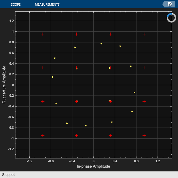
Adjust the memoryless nonlinearity object configuration to add a small AM-PM conversion impairment. AM-PM conversion is a nonlinear impairment that distorts symbols more as the distance from the origin increases. The AM-PM conversion causes the constellation to rotate.
Pass the modulated signal through the nonlinear amplifier, and then plot constellation diagram to show the combined AM-AM and AM-PM distortion.
mnlamp.PhaseGainRadian = pi/9;
mnlampSig = mnlamp(modSig);
constDiagram(mnlampSig)
release(constDiagram)
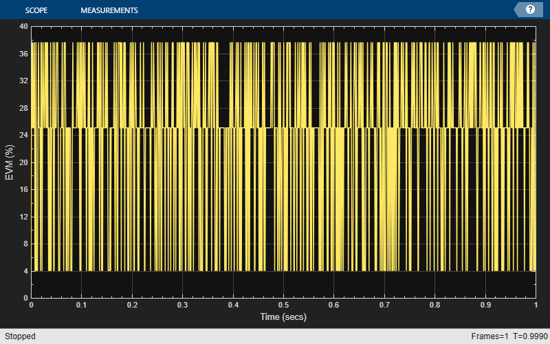
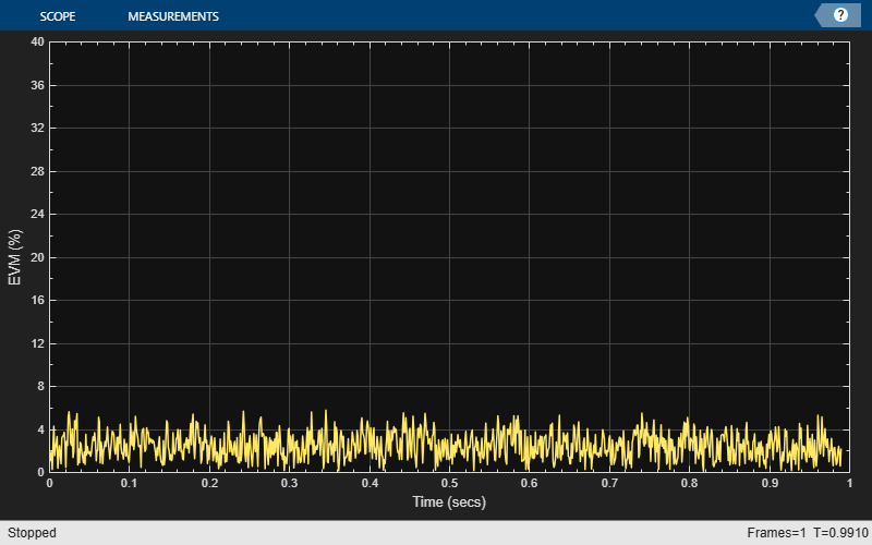
Configure an EVM object to input the reference signal source as an input argument and to average results across rows of the signal. Estimating the EVM against the input signal provides more accurate results. Averaging results across rows of the signal computes the time-varying EVM.
evm = comm.EVM(AveragingDimensions=2);
Plot the time-varying EVM of the distorted signal.
evmTime = evm(modSig,mnlampSig);
timeScope(evmTime)
release(timeScope)
Compute the RMS EVM.
evmRMS = sqrt(mean(evmTime.^2))
evmRMS =
26.4586
Estimate the SNR of the signal after adding the amplifier distortion by using an MER object.
mer = comm.MER;
snrEst = mer(modSig,mnlampSig)
snrEst =
10.1342
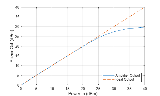
Measure the amplifier output power over a range of input power levels. Specify input power levels ranging from 0 to 40 dBm. Convert those levels to their linear equivalent in watts. Initialize the output power vector.
powerIn = 0:40;
pin = 10.^((powerIn-30)/10);
powerOut = zeros(length(powerIn),1);
for k = 1:length(powerIn)
    data = randi([0 15],1000,1);
    txSig = qammod( ...
        data,16,UnitAveragePower=true)*sqrt(pin(k));
    mnlampSig = mnlamp(txSig);
    powerOut(k) = 10*log10(var(mnlampSig))+30;
end
Plot the power output versus power input curve. The output power levels off at 30 dBm. The amplifier exhibits nonlinear behavior for input power levels greater than 22 dBm.
figure
plot(powerIn,powerOut,powerIn,powerIn,"--")
legend("Amplifier Output","Ideal Output",location="se")
xlabel("Power In (dBm)")
ylabel("Power Out (dBm)")
grid
IQ Imbalance
Apply an amplitude and phase imbalance to the modulated signal using the iqimbal function. The magnitude and phase of the constellation points change linearly as a result of the IQ imbalance.
ampImb = 3;
phImb = 10;
rxSig = iqimbal(modSig,ampImb,phImb);
Plot the IQ imbalance impaired signal constellation diagram and the time-varying EVM.
constDiagram(rxSig)
release(constDiagram)
The time-varying EVM behavior for an IQ imbalance impaired signal is similar to but has less variance than the time-varying EVM behavior due a nonlinear amplifier.
evmTime = evm(modSig,rxSig);
timeScope(evmTime)
release(timeScope)
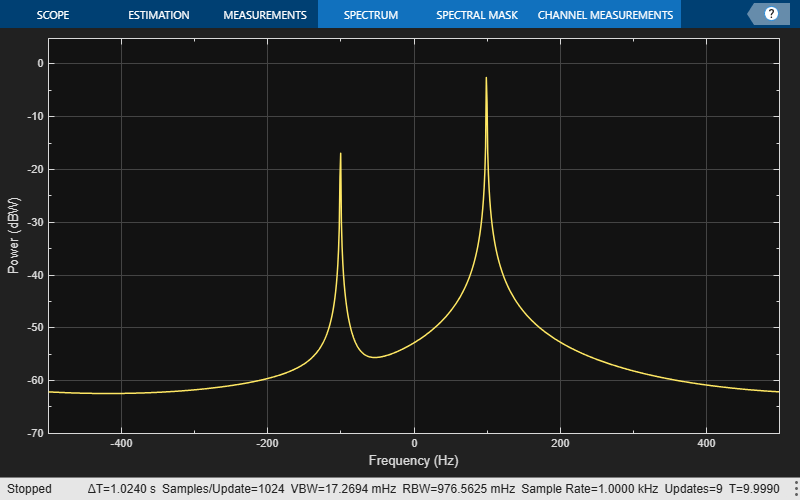
Demonstrate IQ imbalance by applying it to a sine wave, and then showing the spectrum of the IQ imbalance impaired sine wave.
Create a 100 Hz sine wave having a 1000 Hz sample rate by using a sine wave System object™.
sinewave = dsp.SineWave( ...
    Frequency=100, ...
    SampleRate=1000, ...
    SamplesPerFrame=1e4, ...
    ComplexOutput=true);
x = sinewave();
Apply the same 3 dB and 10 degree IQ imbalance.
ampImb = 3;
phImb = 10;
y = iqimbal(x,ampImb,phImb);
Plot the spectrum of the imbalanced signal. The IQ imbalance introduces a second tone at -100 Hz, which is the inverse of the input tone.
spectrum = spectrumAnalyzer( ...
    SampleRate=1000, ...
    SpectrumUnits="dBW");
spectrum(y)
release(spectrum)
Phase Noise
Apply phase noise to the transmitted signal by using a phase noise System object™. The phase noise introduces a rotational jitter.
pnoise = comm.PhaseNoise( ...
    Level=-50, ...
    FrequencyOffset=20, ...
    SampleRate=fs);
pnoiseSig = pnoise(modSig);
Plot the phase noise impaired signal constellation diagram and the time-varying EVM.
constDiagram(pnoiseSig)
release(constDiagram)
evmTime = evm(modSig,pnoiseSig);
timeScope(evmTime)
release(timeScope)
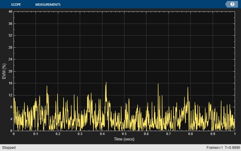
Compute the RMS EVM.
evmRMS = sqrt(mean(evmTime.^2))
evmRMS =
4.9822
Filter Effects
Create a pair of raised cosine matched filters by using the raised cosine transmit and receiver filter System objects. Specify the samples per symbol parameter.
sps = 4;
txfilter = comm.RaisedCosineTransmitFilter( ...
    RolloffFactor=0.2, ...
    FilterSpanInSymbols=8, ...
    OutputSamplesPerSymbol=sps, ...
    Gain=sqrt(sps));
rxfilter = comm.RaisedCosineReceiveFilter( ...
    RolloffFactor=0.2, ...
    FilterSpanInSymbols=8, ...
    InputSamplesPerSymbol=sps, ...
    Gain=1/sqrt(sps), ...
    DecimationFactor=sps);
Determine the delay through the matched filters.
fltDelay = 0.5*( ...
    txfilter.FilterSpanInSymbols + ...
    rxfilter.FilterSpanInSymbols);
Pass the modulated signal through the matched filters.
filtSig = txfilter(modSig);
rxSig = rxfilter(filtSig);
To account for the delay through the filters, discard the first fltDelay samples.
rxSig = rxSig(fltDelay+1:end);
To accommodate the change in the number of received signal samples, create new constellation diagram and time scope objects. Create an EVM object to estimate the EVM.
constDiagram = comm.ConstellationDiagram(ReferenceConstellation=refConst);
timeScope = timescope( ...
    YLimits=[0 40], ...
    SampleRate=fs, ...
    TimeSpanSource="property", ...
    TimeSpan=1, ...
    ShowGrid=true, ...
    YLabel="EVM (%)");
evm = comm.EVM( ...
    ReferenceSignalSource="Estimated from reference constellation", ...
    ReferenceConstellation=refConst, ...
    Normalization="Average constellation power", ...
    AveragingDimensions=2);
Plot the filtered signal constellation diagram and the time-varying EVM.
constDiagram(rxSig)
release(constDiagram)

evmTime = evm(rxSig);
timeScope(evmTime)
release(timeScope)
Compute the RMS EVM.
evmRMS = sqrt(mean(evmTime.^2))
evmRMS =
2.7199
Estimate the SNR by using an MER object.
mer = comm.MER;
snrEst = mer(modSig(1:end-fltDelay),rxSig)
snrEst =
31.4603
White Noise
Pass the 16-QAM signal through an AWGN channel, and then plot its constellation diagram.
noisySig = awgn(modSig,snrdB);
constDiagram(noisySig)
release(constDiagram)
Estimate the EVM of the noisy signal from the reference constellation points.
evm = comm.EVM( ...
    ReferenceSignalSource="Estimated from reference constellation", ...
    ReferenceConstellation=refConst, ...
    Normalization="Average constellation power");
rmsEVM = evm(noisySig)
rmsEVM =
3.1884
The MER measurement corresponds closely to the SNR. Create an MER object, and estimate the SNR. The estimate is close to the specified SNR of 30 dB.
mer = comm.MER( ...
    ReferenceSignalSource="Estimated from reference constellation", ...
    ReferenceConstellation=refConst);
snrEst = mer(noisySig)
snrEst =
30.0754
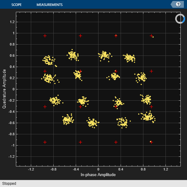
Combined Effects
Combine the effects of the filters, nonlinear amplifier, IQ imbalance, phase noise, and AWGN. Display the constellation diagram, EVM plot, and computed EVM.
Create nonlinear amplifier, phase noise, EVM, time scope, and constellation diagram objects.
mnlamp = comm.MemorylessNonlinearity(Method="Modified Rapp model", ...
    Smoothness=1.4, PhaseGainRadian = pi/9);
pnoise = comm.PhaseNoise(Level=-55,FrequencyOffset=20,SampleRate=fs);
evm = comm.EVM( ...
    ReferenceSignalSource="Estimated from reference constellation", ...
    ReferenceConstellation=refConst, ...
    Normalization="Average constellation power", ...
    AveragingDimensions=2);
timeScope = timescope( ...
    YLimits=[0 40], ...
    SampleRate=fs, ...
    TimeSpanSource="property", ...
    TimeSpan=1, ...
    ShowGrid=true, ...
    YLabel="EVM (%)");
constDiagram = comm.ConstellationDiagram( ...
    ReferenceConstellation=refConst);
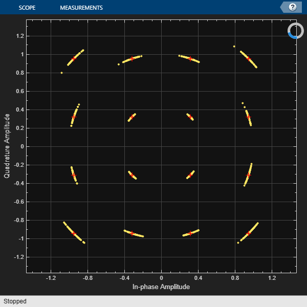
Apply transmitter filtering, and then amplify the modulated signal. Add IQ imbalance and phase noise.
txfiltOut = txfilter(modSig);
mnlampSig = mnlamp(txfiltOut);
iqImbalSig = iqimbal(mnlampSig,ampImb,phImb);
txSig = pnoise(iqImbalSig);
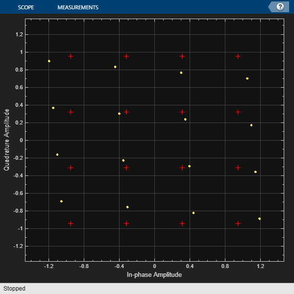
Pass the impaired signal through the AWGN channel. Plot the constellation diagram.
rxSig = awgn(txSig,snrdB);
rxfiltOut = rxfilter(rxSig);

constDiagram(rxfiltOut)
release(constDiagram)
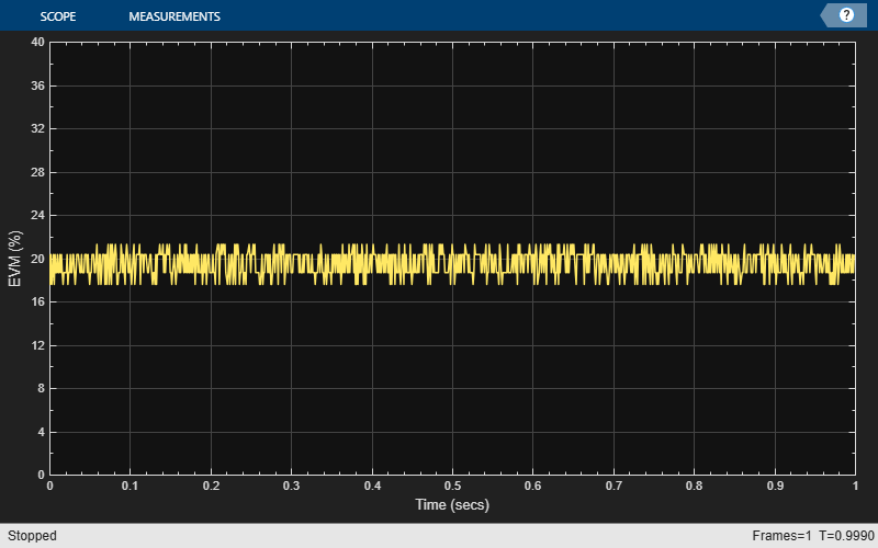
Calculate the time-varying EVM. Plot the result.
evmTime = evm(rxfiltOut);
timeScope(evmTime)
release(timeScope)
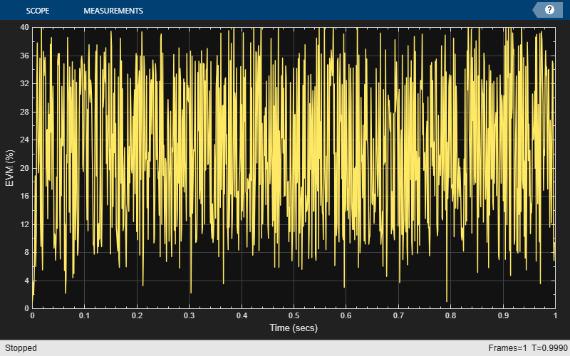
Determine the RMS EVM.
evmRMS = sqrt(mean(evmTime.^2))
evmRMS =
24.4763
Estimate the SNR. This value is approximately 20 dB worse than the specified value of 30 dB. This level of RF impairment effects is significant and will likely degrade the bit error rate performance if it is not corrected by impairment compensation or an advanced receiver.
mer = comm.MER( ...
    ReferenceSignalSource="Estimated from reference constellation", ...
    ReferenceConstellation=refConst);
snrEst = mer(rxfiltOut)
snrEst =
9.6945
See Also
Fading Channels | Impact of RF Effects on Communication System Performance