psample

Sample linear parameter-varying or time-varying dynamics

Since R2024a

Syntax

ssArray = psample(vSys,T)

ssArray = psample(vSys,T,P)

ssArray = psample(vSys,T,P1,...,Pn)

ssArray = psample(vSys,S)

ssArray = psample(vSys)

Description

ssArray = psample(vSys,T) samples the dynamics of the linear time-varying (LTV) model vSys at the times specified in the time vector T and returns an array of time-invariant state-space (ss) models.

ssArray = psample(vSys,T,P) samples the dynamics of the linear-parameter varying (LPV) model vSys at the single point (T,P) and returns an array of time-invariant state-space (ss) models. Set T to [] if the dynamics of the LPV model only depend on P.

ssArray = psample(vSys,T,P1,...,Pn) samples the dynamics over a grid of (T,P) values. P1,...,Pn are arrays specifying the values of each parameter of the LPV model.

ssArray = psample(vSys,S) specifies the sample values as a structure S.

ssArray = psample(vSys) samples a gridded LTV or LPV model at values obtained from vSys.Grid. You can use this syntax as a quick way to access the state-space data and offsets used to construct the gridded LTV or LPV model.

Examples

Sample Dynamics of LTV Models

You can sample the dynamics of an LTV model over a point or a vector of $\mathit{t}$ values to obtain affine dynamics for a given time.

Consider a model defined by the data function ltvssDataFcn.m.

Create an LTV model.

ltvSys = ltvss(@ltvssDataFcn)

Continuous-time state-space LTV model with 1 outputs, 1 inputs, and 1 states.

Define a set of times values to sample this model over.

t = 5:0.5:10;

Use the psample command to obtain an array of ss models.

ssArray = psample(ltvSys,t);
size(ssArray)

1x11 array of state-space models.
Each model has 1 outputs, 1 inputs, and 1 states.

In ssArray, the SamplingGrid property tracks the dependence of each model on time and the Offsets property contains the offset values as a function of time.

ssArray.SamplingGrid

ans = struct with fields:
    Time: [5 5.5000 6 6.5000 7 7.5000 8 8.5000 9 9.5000 10]

ssArray.Offsets

ans=1×11 struct array with fields:
    dx
    x
    u
    y

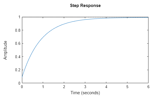
Plot the step response of the fourth model in the array.

step(ssArray(:,:,:,4))

View the data function.

type ltvssDataFcn.m

function [A,B,C,D,E,dx0,x0,u0,y0,Delays] = ltvssDataFcn(t)
% SISO, first order
A = -(1+0.5*sin(t));
B = 1;
C = 1;
D = 0;
E = [];
dx0 = [];
x0 = [];
u0 = [];
y0 = 0.1*sin(5*t);
Delays = [];

Sample Dynamics of LPV Models

You can sample the dynamics of an LPV model over a point or a grid of ($\mathit{t}$,$\mathit{p}$) values to obtain affine dynamics for a given time or parameter value.

For this example, dataFcnMaglev.m defines the matrices and offsets of a magnetic levitation system. The magnetic levitation controls the height of a levitating ball using a coil current that creates a magnetic force on the ball.

Create an LPV model.

lpvSys = lpvss('h',@dataFcnMaglev)

Continuous-time state-space LPV model with 1 outputs, 1 inputs, 2 states, and 1 parameters.

Sample the LPV dynamics at three h values to obtain local LTI models.

hmin = 0.05;
hmax = 0.25;
hcd = linspace(hmin,hmax,3);
ssArray = psample(lpvSys,[],hcd);
size(ssArray)

1x3 array of state-space models.
Each model has 1 outputs, 1 inputs, and 2 states.

The function stores the model offsets in the Offsets property of the array.

ssArray.Offsets

ans=1×3 struct array with fields:
    dx
    x
    u
    y

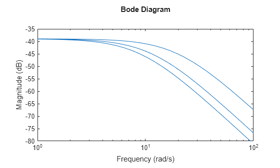
Plot the Bode response.

bodemag(ssArray)

View the data function.

type dataFcnMaglev.m

function [A,B,C,D,E,dx0,x0,u0,y0,Delays] = dataFcnMaglev(~,p)
% MAGLEV example:
% x = [h ; dh/dt]
% p=hbar (equilibrium height)
mb = 0.02; % kg
g = 9.81;
alpha = 2.4832e-5;
A = [0 1;2*g/p 0];
B = [0 ; -2*sqrt(g*alpha/mb)/p];
C = [1 0];  % h
D = 0;
E = [];
dx0 = [];
x0 = [p;0];
u0 = sqrt(mb*g/alpha)*p;  % ibar
y0 = p;                   % y = h = hbar + (h-hbar)
Delays = [];

Sample LPV Dynamics Over Grid Values Specified Using Structures

This example shows how to specify sampling grid values using a structure array.

For this example, lpvHCModel.m defines the following model.

$$\dot{\mathit{x}}=-\left(\mathit{x}-{\mathit{x}}_0\left(\mathit{p}\right)\right)+\left(\mathit{u}-{\mathit{u}}_0\left(\mathit{p}\right)\right)$$

$$\mathit{y}={\mathit{y}}_0\left(\mathit{p}\right)+\left(1-{\mathit{p}}^2\right)\left(\mathit{x}-{\mathit{x}}_0\left(\mathit{p}\right)\right)$$

$\left({\mathit{x}}_0\left(\mathit{p}\right),{\mathit{u}}_0\left(\mathit{p}\right),{\mathit{y}}_0\left(\mathit{p}\right)\right)=\left({\tanh }^{-1}\left(\mathit{p}\right),{\tanh }^{-1}\left(\mathit{p}\right),\mathit{p}\right)$

Use lpvss to construct this LPV plant. Since ${\tanh }^{-1}\left(\mathit{p}\right)$ is infinite for $\left|\mathit{p}\right|=1$, clip $\mathit{p}$ to the range [–0.99,0.99] to stay away from the singularity.

pmax = 0.99;
G = lpvss('p',@(t,p) lpvHCModel(t,p,pmax),'StateName','x')

Continuous-time state-space LPV model with 1 outputs, 1 inputs, 1 states, and 1 parameters.

Specify a structure containing the sampling values.

pvals = linspace(-0.9,0.9,5);
S = struct('p',pvals)

S = struct with fields:
    p: [-0.9000 -0.4500 0 0.4500 0.9000]

Sample the model.

ssArr = psample(G,S);
size(ssArr)

1x5 array of state-space models.
Each model has 1 outputs, 1 inputs, and 1 states.

View the data function.

type lpvHCModel.m

function [A,B,C,D,E,dx0,x0,u0,y0,Delays] = lpvHCModel(~,p,pmax) 
% Plant model

p = max(-pmax,min(p,pmax));
tau = atanh(p);

A = -1;
B = 1;
C = 1-p^2;
D = 0;
E = [];
dx0 = [];
x0 = tau;
u0 = tau;
y0 = p;
Delays = [];

Obtain State-Space Data from Gridded Model

You can obtain the array of state-space models back from the gridded LTV or LPV model using the psample command.

For this example, load a gridded LPV model obtained from the batch linearization of a water-tank Simulink® model in the Create LPV Model from Batch Linearization Results example.

load watertankLPVModel.mat

Obtain the array of local state-space models.

ssArray = psample(gLPV);
size(ssArray)

7x1 array of state-space models.
Each model has 1 outputs, 1 inputs, and 1 states.

For a gridded model, the psample command samples the model at the grid obtained from the Grid property of the model.

gLPV.Grid

ans = struct with fields:
    H: [7x1 double]

Input Arguments

vSys — Varying model to sample

ltvss object | lpvss object

Varying model to sample, specified as an ltvss or lpvss object.

T — Time values

scalar | vector | array

Time values at which the model is sampled.

• For LTV models, specify T as a scalar or vector for real and finite values to sample the dynamics at a single time value or multiple ones, respectively.

• For LPV models, specify T as one of the following:

  • [] — LPV model dynamics only depend only on parameters p.

  • Scalar — Sample the dynamics at a single time value.

  • Vector — Sample the dynamics at multiple time values.

  • Multidimensional array — Sample the dynamics at a grid of values. To specify a rectangular (T,P) grid of values, use ndgrid.

    [t,p1,p2,p3] = ndgrid(tvals,p1vals,p2vals,p3vals)

  The vectors or arrays T and P1,...,Pn must be of the same size.

In discrete time, specify T as integer index values k that count the number of sampling periods Ts. The absolute time is given by t = k*Ts.

P — Parameter values

scalar | vector | array

Parameter values at which the LPV model is sampled.

For an LPV model with n parameters, use comma-separated arguments P1,...,Pn to specify the values for each parameter.

Specify P as one of the following:

• Scalar — Sample the dynamics at a single parameter value.

• Vector — Sample the dynamics at multiple parameter values.

• Multidimensional array — Sample the dynamics at a grid of values. For example, to specify a rectangular (T,P) grid of values, you can use ndgrid.

  [t,p1,p2,p3] = ndgrid(tvals,p1vals,p2vals,p3vals)

  The vectors or arrays T and P1,...,Pn must be of the same size.

S — Sampling grid structure

struct

Sampling grid structure array used to specify values at which the model is sampled.

• For LTV models, S is a structure array with field Time. For example, if an array Tvalues specifies the sampling time, S is the following structure.

  S = struct('Time',Tvalues)

• For LPV models, S is a structure with fields for parameter names corresponding to the ParameterName property of the lpvss model vSys and Time. For example, if vSys has two parameters named 'speed' and 'altitude' with values specified using arrays P1vals and P2vals, respectively, S is the following structure.

  S = struct('speed',P1vals,'altitude',P2vals)

  If the dynamics of your LPV model depend on parameter values, do not specify the field Time for S.

Output Arguments

ssArray — Sampled dynamics

array of ss models

Sampled dynamics, returned as an array of time-invariant state-space (ss) models.

For this array, the SamplingGrid property tracks the dependence of each model on T and P values and the Offsets property contains the offset values as a function of T and P values.

The dimensions of ssArray depend on the number of sampling points in the array or grid.

Version History

Introduced in R2024a

R2024a: Recommended over sample

psample has better support for model offsets and stores them directly in the Offsets property of the state-space model array.