dss2ss

R2026b

Convert descriptor state-space model to explicit form

Since R2024a

Syntax

sys = dss2ss(dsys)

sys = dss2ss(dsys,"consistent")

[sys,info] = dss2ss(dsys,info)

Description

sys = dss2ss(dsys) eliminates the E matrix in the descriptor state-space model (or model array) dsys of the form

$$\begin{array}{l}E\dot{x}=Ax+Bu\\ y=Cx+Du\end{array}$$

and returns an explicit state-space model (or model array) sys of the form

$$\begin{array}{l}{\dot{x}}_e=A_e{x}_e+B_{e}u\\ y=C_e{x}_e+D_{e}u\end{array}$$

Here, dsys must be proper and the number of states x_e in sys is smaller than number of states x in dsys when E is singular (the explicit form removes the algebraic variables). Use findop to compute matching initial conditions when the state is reduced.

sys = dss2ss(dsys,"consistent") takes an array of descriptor state-space models dsys and eliminates E while preserving state consistency, that is, all models in sys share the same state vector x. This requires all E matrices to be invertible. The "consistent" argument has no effect if dsys is a single model instead of a model array.

[sys,info] = dss2ss(dsys,info) takes a single descriptor state-space models dsys and an info matrix or structure containing projection and initial condition information to propagate through the transformation. It also returns the updated info structure as second output. For more information on projector matrices, see Spectral Projector Matrices.

Examples

Convert Descriptor State-Space Model to Explicit Form

This example shows how to use dss2ss to convert a state-space model in descriptor form to explicit form.

For this example, consider a cube rotating about its corner with inertia tensor J and a damping force F of 0.2 magnitude. The input to the system is the driving torque while the angular velocities are the outputs. The equation is given by:

$$J\frac{d\omega }{\text{dt}}+F\omega =T$$

$$y=\omega$$

The state-space matrices for the cube are:

$$\begin{array}{l}A=-F,B=I,C=I,D=0,E=J,\\ where,J=\left[\begin{array}{ccc}8& -3& -3\\ -3& 8& -3\\ -3& -3& 8\end{array}\right]andF=\left[\begin{array}{ccc}0.2& 0& 0\\ 0& 0.2& 0\\ 0& 0& 0.2\end{array}\right]\end{array}$$

Specify the A, B, C and D matrices, and create the continuous-time descriptor state-space model.

J = [8 -3 -3; -3 8 -3; -3 -3 8];
F = 0.2*eye(3);
A = -F;
B = eye(3);
C = eye(3);
D = 0;
E = J;
dsys = dss(A,B,C,D,E);

To convert this model to explicit form, use dss2ss. Also return the info structure as second output argument.

[esys,info] = dss2ss(dsys);
esys.E

ans =

     []

As you can see, the $E$ matrix is empty.

sigma(dsys,esys,'r--')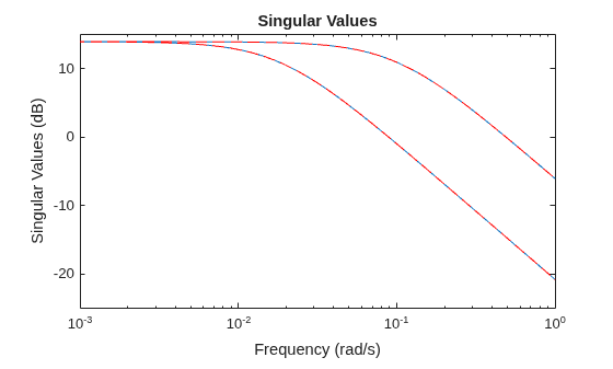

The singular values plot shows that dsys and esys are equivalent.

Propagate Initial Condition and Projection Matrices from Descriptor to Explicit Form

Load the descriptor state space system dsys and its initial condition from the supporting file dss2ss_prop.mat.

load dss2ss_prop.mat

Display some system information.

size(dsys)

State-space model with 1 outputs, 1 inputs, and 7 states.

rank(dsys.E)

ans = 
6

damp(dsys)

                                                                       
         Pole              Damping       Frequency      Time Constant  
                                       (rad/seconds)      (seconds)    
                                                                       
 -1.00e+00                 1.00e+00       1.00e+00         1.00e+00    
 -8.41e-01 + 2.30e+00i     3.43e-01       2.45e+00         1.19e+00    
 -8.41e-01 - 2.30e+00i     3.43e-01       2.45e+00         1.19e+00    
 -8.32e+00                 1.00e+00       8.32e+00         1.20e-01    

Display the initial condition.

x0d

x0d = 7×1

  -17.6777
    7.5216
   -1.0547
    1.2629
    1.0682
    0.4389
   -0.1845

Convert the system to explicit state space form.

[sys,info] = dss2ss(dsys,x0d); 

Display some system information.

size(sys)

State-space model with 1 outputs, 1 inputs, and 4 states.

Display the equivalent initial condition.

info.InitialCondition

ans = 4×1

  164.8761
   35.6971
   12.6964
   40.6659

You can obtain this initial condition by propagating the original initial condition x0d through the state projection matrix.

info.PX'*x0d

ans = 4×1

  164.8761
   35.6971
   12.6964
   40.6659

For more information, see Spectral Projector Matrices.

To compare the initial responses, use the initial function.

t = linspace(0,10,100);
initial(dsys,x0d,t);
hold on
initial(sys,info.PX'*x0d,t,'--');

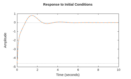
The response is identical, confirming that info.InitialCondition is equivalent to x0d.

Input Arguments

dsys — Descriptor state-space model

ss object | ss object array

Descriptor state-space model, specified as a state-space model or an array of state-space models.

info — Projection and initial condition information to propagate trough the transformation

vector | matrix | structure

Information to propagate trough the transformation, specified as either a matrix (possibly a column vector) in which each column contains an initial condition for dsys, or as a structure containing the following fields:

• PL — A left projector matrix

• PR — A right projector matrix

• PX — A state-space transformation matrix

• InitialCondition — A matrix in which each column contains an initial condition for dsys.

For more information on projector matrices, see Spectral Projector Matrices in the algorithm section of getrom.

When transforming the dsys descriptor state-space model into the explicit state-space model sys, the dss2ss function also propagates the same transformation to the projection matrices and to the initial condition vector. The function places the updated projection matrices and the corresponding initial condition in the updated info structure that is returned as last output argument.

When info is a matrix of initial conditions instead of a structure, dss2ss propagates the transformation to the initial condition vectors, and returns the updated initial conditions (along with the new projection matrices that define the transformation enacted by dss2ss) in the updated info structure that is returned as second output argument.

Note that the presence of offsets and initial conditions influences the input-to-state map and therefore affects which states can be safely removed.

Output Arguments

sys — Explicit state-space model

ss object | ss object array

Explicit state-space model, returned as a state-space model or an array of state-space models.

info — Updated projection and initial condition information

structure

Updated projection and initial condition information, returned as a structure.

The structure contains the following fields:

• PL — A left projector matrix

• PR — A right projector matrix

• PX — A state-space transformation matrix

• InitialCondition — A vector of initial conditions for sys.

For more information on projector matrices, see Spectral Projector Matrices in the algorithm section of getrom.

When info is returned as output from the sminreal function, it also contains the following fields:

• ekeep — A logical vector indicating which state equations are retained.

• PR — A logical vector indicating which internal delays are retained.

• PX — A logical vector indicating which blocks (for LFT systems only) are retained.

Version History

Introduced in R2024a