Time-Domain Response Data and Plots

This example shows how to obtain step and impulse response data, as well as step and impulse response plots, from a dynamic system model.

Create a transfer function model and plot its response to a step input at $$t$$ = 0.

H = tf([8 18 32],[1 6 14 24]);
step(H);

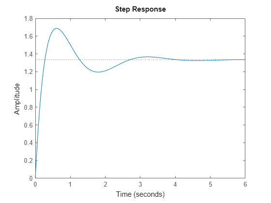
When call step without output arguments, it plots the step response on the screen. Unless you specify a time range to plot, step automatically chooses a time range that illustrates the system dynamics.

Calculate the step response data from $$t$$ = 0 (application of the step input) to $$t$$ = 8 s.

[y,t] = step(H,8);

When you call step with output arguments, the command returns the step response data y. The vector t contains corresponding time values.

Plot the response of H to an impulse input applied at $$t$$ = 0. Plot the response with a grid.

opts = timeoptions;
opts.Grid = 'on';
impulseplot(H,opts)

Use the timeoptions command to define options sets for customizing time-domain plots with commands like impulseplot and stepplot.

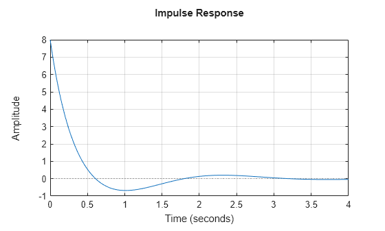
Calculate 200 points of impulse response data from $$t$$ = 1 (one second after application of the impulse input) to $$t$$ = 3s.

[y,t] = impulse(H,linspace(1,3,200));

As for step, you can omit the time vector to allow impulse to automatically select a time range.