predint
Prediction intervals for cfit or sfit object
Syntax
Description
ci = predint(fitresult,x)cfit object fitresult at the new predictor values specified by the vector x. fitresult must be an output from the fit function to contain the necessary information for ci. ci is an n-by-2 array where n = length(x). The left column of ci contains the lower bound for each coefficient; the right column contains the upper bound.
ci = predint(fitresult,x,level,intopt,simopt)
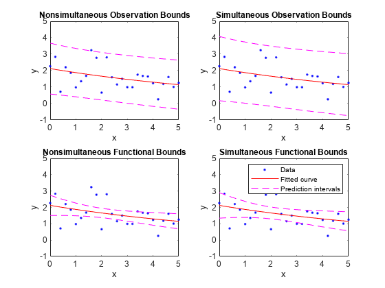
Observation bounds are wider than functional bounds because they measure the uncertainty of predicting the fitted curve plus the random variation in the new observation. Non-simultaneous bounds are for individual elements of x; simultaneous bounds are for all elements of x.
Examples
Calculate and plot observation and functional prediction intervals for a fit to noisy data.
Generate noisy data with an exponential trend.
x = (0:0.2:5)';
y = 2*exp(-0.2*x) + 0.5*randn(size(x));
Fit a curve to the data using a single-term exponential.
fitresult = fit(x,y,'exp1');Compute 95% observation and functional prediction intervals, both simultaneous and nonsimultaneous. Nonsimultaneous bounds are for individual elements of x; simultaneous bounds are for all elements of x.
p11 = predint(fitresult,x,0.95,'observation','off');
p12 = predint(fitresult,x,0.95,'observation','on');
p21 = predint(fitresult,x,0.95,'functional','off');
p22 = predint(fitresult,x,0.95,'functional','on');
Plot the data, fit, and prediction intervals. Observation bounds are wider than functional bounds because they measure the uncertainty of predicting the fitted curve plus the random variation in the new observation.
subplot(2,2,1)
plot(fitresult,x,y), hold on, plot(x,p11,'m--'), xlim([0 5]), ylim([-1 5])
title('Nonsimultaneous Observation Bounds','FontSize',9)
legend off

subplot(2,2,2)
plot(fitresult,x,y), hold on, plot(x,p12,'m--'), xlim([0 5]), ylim([-1 5])
title('Simultaneous Observation Bounds','FontSize',9)
legend off

subplot(2,2,3)
plot(fitresult,x,y), hold on, plot(x,p21,'m--'), xlim([0 5]), ylim([-1 5])
title('Nonsimultaneous Functional Bounds','FontSize',9)
legend off

subplot(2,2,4)
plot(fitresult,x,y), hold on, plot(x,p22,'m--'), xlim([0 5]), ylim([-1 5])
title('Simultaneous Functional Bounds','FontSize',9)
legend({'Data','Fitted curve', 'Prediction intervals'},...
       'FontSize',8,'Location','northeast')
Input Arguments
Output Arguments
Limitations
Prediction intervals cannot be computed for fit objects with constraint points
specified. The software will return NaN values.
Version History
Introduced in R2013a