Chebyshev (a.k.a. Equioscillating) Spline Defined

By definition, for given knot sequence t of length n+k, C = C_{t,k} is the unique element of S_{t,k} of max-norm 1 that maximally oscillates on the interval [t_k .. t_{n+1}] and is positive near t_{n+1}. This means that there is a unique strictly increasing tau of length n so that the function C in S_{k,t} given by

C(tau(i)) = (-1)^{n-i},

for all i, has max-norm 1 on [t_k .. t_{n+1}]. This implies that

tau(1) = t_k,

tau(n) = t_{n+1},

and that

t_i < tau(i) < t_{k+i},

for all i. In fact,

t_{i+1} <= tau(i) <= t_{i+k-1},

for all i. This brings up the point that the knot sequence t is assumed to make such an inequality possible, which turns out to be equivalent to having all the elements of S_{k,t} continuous.

t = augknt([0 1 1.1 3 5 5.5 7 7.1 7.2 8], 4 );
[tau,C] = chbpnt(t,4);
xx = sort([linspace(0,8,201),tau]);
plot(xx,fnval(C,xx),'LineWidth',2);
hold on
breaks = knt2brk(t); 
bbb = repmat(breaks,3,1);
sss = repmat([1;-1;NaN],1,length(breaks));
plot(bbb(:), sss(:),'r');
hold off
ylim([-2 2]);
title('The Chebyshev Spline for a Particular Knot Sequence');
legend({'Chebyshev Spline' 'Knots'});

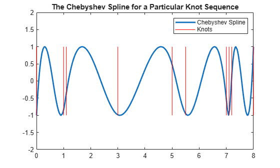
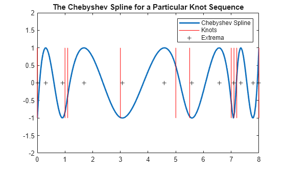
In short, the Chebyshev spline C looks just like the Chebyshev polynomial. It performs similar functions. For example, its extrema tau are particularly good sites to interpolate at from S_{k,t} since the norm of the resulting projector is about as small as can be.

hold on
plot(tau,zeros(size(tau)),'k+');
hold off
legend({'Chebyshev Spline' 'Knots' 'Extrema'});

Choice of Spline Space

In this example, we try to construct C for a given spline space.

We deal with cubic splines with simple interior knots, specified by

k = 4;
breaks = [0 1 1.1 3 5 5.5 7 7.1 7.2 8];
t = augknt(breaks, k)

t = 1×16

         0         0         0         0    1.0000    1.1000    3.0000    5.0000    5.5000    7.0000    7.1000    7.2000    8.0000    8.0000    8.0000    8.0000

thus getting a spline space of dimension

n = length(t)-k

n = 12

Initial Guess

As our initial guess for the tau, we use the knot averages

tau(i) = (t_{i+1} + ... + t_{i+k-1})/(k-1)

recommended as good interpolation site choices, and plot the resulting first approximation to C.

tau = aveknt(t,k)

tau = 1×12

         0    0.3333    0.7000    1.7000    3.0333    4.5000    5.8333    6.5333    7.1000    7.4333    7.7333    8.0000

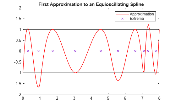
b = (-ones(1,n)).^(n-1:-1:0);
c = spapi(t,tau,b);
plot(breaks([1 end]),[1 1],'k', breaks([1 end]),[-1 -1],'k');
hold on
fnplt(c,'r',1);
hold off
ylim([-2 2]);
title('First Approximation to an Equioscillating Spline');

Iteration

For the complete leveling, we use the Remez algorithm. This means that we construct a new tau as the extrema of our current approximation, c, to C and try again.

Finding these extrema is itself an iterative process, namely, for finding the zeros of the derivative Dc of our current approximation c.

Dc = fnder(c);

We take the zeros of the control polygon of Dc as our first guess for the zeros of Dc. This control polygon has the vertices (tstar(i),coefs(i)), where coefs are the coefficients of Dc, and tstar the knot averages.

[knots,coefs,np,kp] = fnbrk(Dc, 'knots', 'coefs', 'n', 'order');
tstar = aveknt(knots,kp);

Since the control polygon is piecewise linear, its zeros are easy to compute. Here are those zeros.

npp = 1:np-1;
guess = tstar(npp) - coefs(npp).*(diff(tstar)./diff(coefs));
fnplt(Dc,'r');
hold on
plot(tstar,coefs,'k.:');
plot(guess,zeros(1,np-1),'o');
hold off
title('First Derivative of the Approximation');
legend({'Dc' 'Control Polygon' 'Zeros of Control Polygon'});

This provides a very good first guess for the actual zeros of Dc.

Now we evaluate Dc at both these sets of sites.

sites = [guess; tau(2:n-1)];
values = fnval(Dc,sites);

Then we use two steps of the secant method, getting iterates sites(3,:) and sites(4,:), with values(3,:) and values(4,:) the corresponding values of Dc.

sites(3:4,:) = 0;
values(3:4,:) = 0;
for j = 2:3
   rows = [j,j-1]; 
   Dcd = diff(values(rows,:));
   Dcd(Dcd==0) = 1; % guard against division by zero
   sites(j+1,:) = sites(j,:)-values(j,:).*(diff(sites(rows,:))./Dcd);
   values(j+1,:) = fnval(Dc,sites(j+1,:));
end

We take the last iterate as the computed zeros of Dc, i.e., the extrema of our current approximation, c. This is our new guess for tau.

tau = [tau(1) sites(4,:) tau(n)]

tau = 1×12

         0    0.2759    0.9082    1.7437    3.0779    4.5532    5.5823    6.5843    7.0809    7.3448    7.7899    8.0000

plot(breaks([1 end]),[1 1],'k', breaks([1 end]),[-1 -1],'k');
hold on
fnplt(c,'r',1);
plot(guess,zeros(1,np-1),'o');
plot(tau(2:n-1),zeros(1,n-2),'x');
hold off
title('First Approximation to an Equioscillating Spline');
ax = gca;
h = ax.Children;
legend(h([3 1 2]),{'Approximation' 'Extrema' ...
                   'Zeros of First Derivative''s Control Polygon'});
axis([0 8 -2 2]);

End of First Iteration Step

We compute the resulting new approximation to the Chebyshev spline using the new guess for tau.

cnew = spapi(t,tau,b);

The new approximation is more nearly an equioscillating spline.

plot(breaks([1 end]),[1 1],'k', breaks([1 end]),[-1 -1],'k');
hold on
fnplt(c,'r',1);
fnplt(cnew, 'k', 1);
hold off
ax = gca;
h = ax.Children;
legend(h([2 1]),{'First Approximation' 'Updated Approximation'});
axis([0 8 -2 2]);

If this is not close enough, simply try again, starting from this new tau. For this particular example, the next iteration already provides the Chebyshev spline to graphic accuracy.

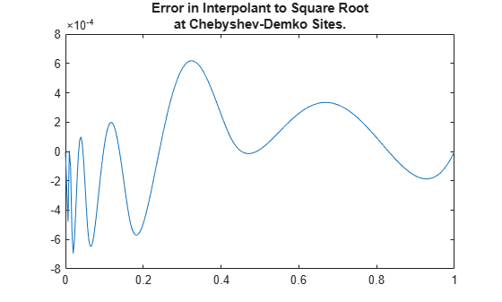
Use of Chebyshev-Demko Points

The Chebyshev spline for a given spline space S_{k,t}, along with its extrema, are available as optional outputs from the chbpnt command in the toolbox. These extrema were proposed as good interpolation sites by Steven Demko, hence are now called the Chebyshev-Demko sites. This section shows an example of their use.

If you have decided to approximate the square-root function on the interval [0 .. 1] by cubic splines with knot sequence

k = 4;
n = 10;
t = augknt(((0:n)/n).^8,k);

then a good approximation to the square-root function from that specific spline space is given by

tau = chbpnt(t,k);
sp = spapi(t,tau,sqrt(tau));

as is evidenced by the near equioscillation of the error.

xx = linspace(0,1,301);
plot(xx, fnval(sp,xx)-sqrt(xx));
title({'Error in Interpolant to Square Root','at Chebyshev-Demko Sites.'});