Fit Polynomial Model to Data
This example shows how to fit a polynomial model to data using the linear least-squares method.
Load the patients data set.
load patientsThe variables Diastolic and Systolic contain data for diastolic and systolic blood pressure measurements, respectively. Fit a third-degree polynomial to the data with Diastolic as the predictor variable and Systolic as the response.
polymodel = fit(Diastolic,Systolic,"poly3")polymodel =
Linear model Poly3:
polymodel(x) = p1*x^3 + p2*x^2 + p3*x + p4
Coefficients (with 95% confidence bounds):
p1 = -0.001061 (-0.003673, 0.001551)
p2 = 0.2844 (-0.3701, 0.9389)
p3 = -24.72 (-79.2, 29.76)
p4 = 821.1 (-685.5, 2328)
polymodel contains the results of the fit. Display the least-squares method used to estimate the coefficients by using the function fitoptions.
opts = fitoptions(polymodel);
opts.Method
ans =
'LinearLeastSquares'
The output shows that polymodel is fit to the data with the linear least-squares method. Evaluate polymodel at the values in Diastolic, and display the result together with a scatter plot of the blood pressure data.
plot(polymodel,Diastolic,Systolic)
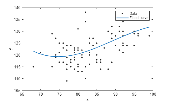
The plot shows that polymodel follows the bulk of the data.