Analyze Relational Database Data
R2026bThis example shows how to navigate, import, and analyze data from a simple DuckDB™ relational database file.
Connect to Database
Connect to the DuckDB™ database file nyctaxi.db in the matlabroot/toolbox/database/dbdata folder by using the duckdb function. Because nyctaxi.db is read-only, open the file by specifying ReadOnly=true. The database contains the table demo used in this workflow.
filePath = fullfile(matlabroot,"toolbox","database","dbdata","nyctaxi.db");
conn = duckdb(filePath,ReadOnly=true);
View Catalogs, Schemas, and Tables
A catalog is the highest-level container in a relational database. It contains schemas that group related tables. Table columns define attributes and data types, and rows store the data values. In this example, each row in the demo table represents a taxi ride in the nyctaxi database.
Inspect the database structure by using the sqlfind function to return metadata, including the column count, table name, schema name, and catalog name. To retrieve metadata for all tables, set the input argument pattern to an empty string.
pattern = "";
sqlfind(conn,pattern)
ans = 1×5 table
Catalog Schema Table Columns Type
_________ ______ ______ _____________________________________________________________________________________________________________________________________________________________________________________________________________________________________________________________________________________________________________________________________________________________________________________ ____________
"nyctaxi" "main" "demo" {["vendorid" "tpep_pickup_datetime" "tpep_dropoff_datetime" "passenger_count" "trip_distance" "pickup_longitude" "pickup_latitude" "ratecodeid" "store_and_fwd_flag" "dropoff_longitude" "dropoff_latitude" "payment_type" "fare_amount" "extra" "mta_tax" "tip_amount" "tolls_amount" "improvement_surcharge" "total_amount"]} "BASE TABLE"
Before importing the data, identify the available columns by retrieving the column names and data types using the fetch function.
tableName = "demo";
sqlQuery = "SELECT column_name, data_type " + ...
    "FROM information_schema.columns " + ...
    "WHERE table_name = '" + tableName + "';";
data = fetch(conn,sqlQuery);
head(data)
          column_name           data_type
    _______________________    ___________

    "vendorid"                 "DOUBLE"
    "tpep_pickup_datetime"     "TIMESTAMP"
    "tpep_dropoff_datetime"    "TIMESTAMP"
    "passenger_count"          "DOUBLE"
    "trip_distance"            "DOUBLE"
    "pickup_longitude"         "DOUBLE"
    "pickup_latitude"          "DOUBLE"
    "ratecodeid"               "DOUBLE"
Import Database Table
Import the demo table into MATLAB.
sqlQuery = 'SELECT * FROM main.demo';
data = fetch(conn,sqlQuery);
head(data)
vendorid tpep_pickup_datetime tpep_dropoff_datetime passenger_count trip_distance pickup_longitude pickup_latitude ratecodeid store_and_fwd_flag dropoff_longitude dropoff_latitude payment_type fare_amount extra mta_tax tip_amount tolls_amount improvement_surcharge total_amount
________ ____________________ _____________________ _______________ _____________ ________________ _______________ __________ __________________ _________________ ________________ ____________ ___________ _____ _______ __________ ____________ _____________________ ____________
2 09-Jun-2015 14:58:55 09-Jun-2015 15:26:41 1 2.63 -73.983 40.73 1 "N" -73.977 40.759 2 18 0 0.5 0 0 0.3 18.8
2 09-Jun-2015 14:58:55 09-Jun-2015 15:02:13 1 0.32 -73.997 40.732 1 "N" -73.994 40.731 2 4 0 0.5 0 0 0.3 4.8
1 09-Jun-2015 14:58:56 09-Jun-2015 16:08:52 2 20.6 -73.983 40.767 2 "N" -73.798 40.645 1 52 0 0.5 10 5.54 0.3 68.34
1 09-Jun-2015 14:58:57 09-Jun-2015 15:12:00 1 1.2 -73.97 40.762 1 "N" -73.969 40.75 1 9 0 0.5 1.96 0 0.3 11.76
2 09-Jun-2015 14:58:58 09-Jun-2015 15:00:49 5 0.49 -73.978 40.786 1 "N" -73.972 40.785 2 3.5 0 0.5 0 0 0.3 4.3
2 09-Jun-2015 14:58:59 09-Jun-2015 15:42:02 1 16.64 -73.97 40.757 2 "N" -73.79 40.647 1 52 0 0.5 11.67 5.54 0.3 70.01
1 09-Jun-2015 14:58:59 09-Jun-2015 15:03:07 1 0.8 -73.976 40.745 1 "N" -73.983 40.735 1 5 0 0.5 1 0 0.3 6.8
2 09-Jun-2015 14:59:00 09-Jun-2015 15:21:31 1 3.23 -73.982 40.767 1 "N" -73.994 40.736 2 16.5 0 0.5 0 0 0.3 17.3
Analyze Taxi Data
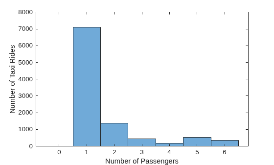
Plot a histogram of the passenger_count column. Most taxi rides had a single passenger.
histogram(data.passenger_count)
xlabel('Number of Passengers')
ylabel('Number of Taxi Rides')
A scatterplot helps visualize the relationship between two variables. For example, plot trip_distance on the x-axis and tip_amount on the y-axis to examine their correlation.
scatter(data{:,"trip_distance"},data{:,"tip_amount"},'o')
xlabel('Trip Distance, miles')
ylabel('Tip Amount, dollars' )
axis([0 50 0 50])
xticks(0:5:50)
yticks(0:5:50)
axis square
box on
grid on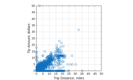
Plot the latitude–longitude pairs from dropoff_latitude and dropoff_longitude on a street basemap to visualize spatial distribution and density. The latlim and lonlim values define a focused view of the New York City area.
latDrop = data{:,"dropoff_latitude"};
lonDrop = data{:,"dropoff_longitude"};
latlim = [40.65 40.85];
lonlim = [-74.0 -73.7];
figure
ax = geoaxes;
geobasemap(ax,'streets');
geoplot(latDrop,lonDrop,'m.','MarkerSize',4)
geolimits(latlim,lonlim)
title({'New York City Drop Off Locations'})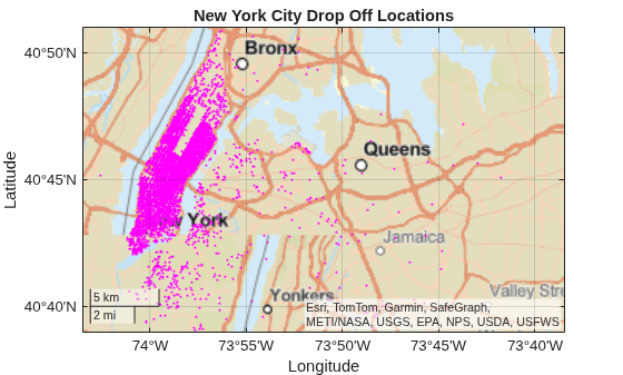
close(conn)

