Dynamical System Modeling Using Neural ODE
This example shows how to train a neural network with neural ordinary differential equations (ODEs) to learn the dynamics of a physical system.
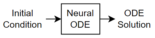
Neural ODEs [1] are deep learning operations defined by the solution of an ODE. More specifically, neural ODE is an operation that can be used in any architecture and, given an input, defines its output as the numerical solution of the ODE
for the time horizon and the initial condition . The right-hand side of the ODE depends on a set of trainable parameters , which the model learns during the training process. In this example, is modeled with a model function containing fully connected operations and nonlinear activations. The initial condition is either the input of the entire architecture, as in the case of this example, or is the output of a previous operation.
This example shows how to train a neural network with neural ODEs to learn the dynamics of a given physical system, described by the following ODE:
,
where is a 2-by-2 matrix.
The neural network of this example takes as input an initial condition and computes the ODE solution through the learned neural ODE model.
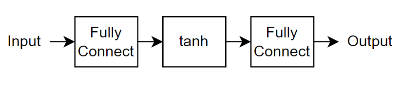
The neural ODE operation, given an initial condition, outputs the solution of an ODE model. In this example, specify a block with a fully connected layer, a tanh layer, and another fully connected layer as the ODE model.
In this example, the ODE that defines the model is solved numerically with the explicit Runge-Kutta (4,5) pair of Dormand and Prince [2]. The backward pass uses automatic differentiation to learn the trainable parameters by backpropagating through each operation of the ODE solver.
The learned function is used as the right-hand side for computing the solution of the same model for additional initial conditions.
Synthesize Data of Target Dynamics
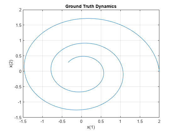
Define the target dynamics as a linear ODE model , with x0 as its initial condition, and compute its numerical solution xTrain with ode45 in the time interval [0 15]. To compute an accurate ground truth data, set the relative tolerance of the ode45 numerical solver to . Later, you use the value of xTrain as ground truth data for learning an approximated dynamics with a neural ODE model.
x0 = [2; 0];
A = [-0.1 -1; 1 -0.1];
trueModel = @(t,y) A*y;

numTimeSteps = 2000;
T = 15;
odeOptions = odeset(RelTol=1.e-7);
t = linspace(0, T, numTimeSteps);
[~, xTrain] = ode45(trueModel, t, x0, odeOptions);
xTrain = xTrain';
Visualize the training data in a plot.
figure
plot(xTrain(1,:),xTrain(2,:))
title("Ground Truth Dynamics")
xlabel("x(1)")
ylabel("x(2)")
grid on
Define and Initialize Model Parameters
The model function consists of a single call to dlode45 to solve the ODE defined by the approximated dynamics for 40 time steps.
neuralOdeTimesteps = 40;
dt = t(2);
timesteps = (0:neuralOdeTimesteps)*dt;
Define the learnable parameters to use in the call to dlode45 and collect them in the variable neuralOdeParameters. The function initializeGlorot takes as input the size of the learnable parameters sz and the number of outputs and number of inputs of the fully connected operations, and returns a dlarray object with underlying type single with values set using Glorot initialization. The function initializeZeros takes as input the size of the learnable parameters, and returns the parameters as a dlarray object with underlying type single. The initialization example functions are attached to this example as supporting files. To access these functions, open this example as a live script. For more information about initializing learnable parameters for model functions, see Initialize Learnable Parameters for Model Function.
Initialize the parameters structure.
neuralOdeParameters = struct;
Initialize the parameters for the fully connected operations in the ODE model. The first fully connected operation takes as input a vector of size stateSize and increases its length to hiddenSize. Conversely, the second fully connected operation takes as input a vector of length hiddenSize and decreases its length to stateSize.
stateSize = size(xTrain,1);
hiddenSize = 20;

neuralOdeParameters.fc1 = struct;
sz = [hiddenSize stateSize];
neuralOdeParameters.fc1.Weights = initializeGlorot(sz, hiddenSize, stateSize);
neuralOdeParameters.fc1.Bias = initializeZeros([hiddenSize 1]);

neuralOdeParameters.fc2 = struct;
sz = [stateSize hiddenSize];
neuralOdeParameters.fc2.Weights = initializeGlorot(sz, stateSize, hiddenSize);
neuralOdeParameters.fc2.Bias = initializeZeros([stateSize 1]);
Display the learnable parameters of the model.
neuralOdeParameters.fc1
ans = struct with fields:
    Weights: [20×2 dlarray]
       Bias: [20×1 dlarray]
neuralOdeParameters.fc2
ans = struct with fields:
    Weights: [2×20 dlarray]
       Bias: [2×1 dlarray]
Define Neural ODE Model
Create the function odeModel, listed in the ODE Model section of the example, which takes as input the time input (unused), the corresponding solution, and the ODE function parameters. The function applies a fully connected operation, a tanh operation, and another fully connected operation to the input data using the weights and biases given by the parameters.
Define Model Function
Create the function model, listed in the Model Function section of the example, which computes the outputs of the deep learning model. The function model takes as input the model parameters and the input data. The function outputs the solution of the neural ODE.
Define Model Loss Function
Create the function modelLoss, listed in the Model Loss Function section of the example, which takes as input the model parameters, a mini-batch of input data with corresponding targets, and returns the loss and the gradients of the loss with respect to the learnable parameters.
Specify Training Options
Specify options for Adam optimization.
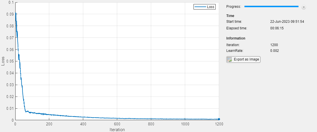
gradDecay = 0.9;
sqGradDecay = 0.999;
learnRate = 0.002;
Train for 1200 iterations with a mini-batch-size of 200.
numIter = 1200;
miniBatchSize = 200;
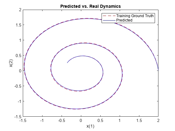
Every 50 iterations, solve the learned dynamics and display them against the ground truth in a phase diagram to show the training path.
plotFrequency = 50;
Train Model Using Custom Training Loop
Initialize the averageGrad and averageSqGrad parameters for the Adam solver.
averageGrad = [];
averageSqGrad = [];
Initialize the TrainingProgressMonitor object. Because the timer starts when you create the monitor object, make sure that you create the object close to the training loop.
monitor = trainingProgressMonitor(Metrics="Loss",Info=["Iteration","LearnRate"],XLabel="Iteration");
Train the network using a custom training loop.
For each iteration:
Construct a mini-batch of data from the synthesized data with the
createMiniBatchfunction, listed in the Create Mini-Batches Function section of the example.Evaluate the model loss and gradients using the
dlfevalfunction and themodelLossfunction, listed in the Model Loss Function section of the example.Update the model parameters using the
adamupdatefunction.Update the training progress plot.
numTrainingTimesteps = numTimeSteps;
trainingTimesteps = 1:numTrainingTimesteps;
plottingTimesteps = 2:numTimeSteps;

iteration = 0;

while iteration < numIter && ~monitor.Stop
    iteration = iteration + 1;

    % Create batch
    [X, targets] = createMiniBatch(numTrainingTimesteps, neuralOdeTimesteps, miniBatchSize, xTrain);

    % Evaluate network and compute loss and gradients
    [loss,gradients] = dlfeval(@modelLoss,timesteps,X,neuralOdeParameters,targets);

    % Update network
    [neuralOdeParameters,averageGrad,averageSqGrad] = adamupdate(neuralOdeParameters,gradients,averageGrad,averageSqGrad,iteration,...
        learnRate,gradDecay,sqGradDecay);

    % Plot loss
    recordMetrics(monitor,iteration,Loss=loss);

    % Plot predicted vs. real dynamics
    if mod(iteration,plotFrequency) == 0  || iteration == 1

        % Use ode45 to compute the solution
        y = dlode45(@odeModel,t,dlarray(x0),neuralOdeParameters,DataFormat="CB");

        plot(xTrain(1,plottingTimesteps),xTrain(2,plottingTimesteps),"r--")

        hold on
        plot(y(1,:),y(2,:),"b-")
        hold off

        xlabel("x(1)")
        ylabel("x(2)")
        title("Predicted vs. Real Dynamics")
        legend("Training Ground Truth", "Predicted")

        drawnow
    end
    updateInfo(monitor,Iteration=iteration,LearnRate=learnRate);
    monitor.Progress = 100*iteration/numIter;
end
Evaluate Model
Use the model to compute approximated solutions with different initial conditions.
Define four new initial conditions different from the one used for training the model.
tPred = t;

x0Pred1 = sqrt([2;2]);
x0Pred2 = [-1;-1.5];
x0Pred3 = [0;2];
x0Pred4 = [-2;0];
Numerically solve the ODE true dynamics with ode45 for the four new initial conditions.
[~, xTrue1] = ode45(trueModel, tPred, x0Pred1, odeOptions);
[~, xTrue2] = ode45(trueModel, tPred, x0Pred2, odeOptions);
[~, xTrue3] = ode45(trueModel, tPred, x0Pred3, odeOptions);
[~, xTrue4] = ode45(trueModel, tPred, x0Pred4, odeOptions);
Numerically solve the ODE with the learned neural ODE dynamics.
xPred1 = dlode45(@odeModel,tPred,dlarray(x0Pred1),neuralOdeParameters,DataFormat="CB");
xPred2 = dlode45(@odeModel,tPred,dlarray(x0Pred2),neuralOdeParameters,DataFormat="CB");
xPred3 = dlode45(@odeModel,tPred,dlarray(x0Pred3),neuralOdeParameters,DataFormat="CB");
xPred4 = dlode45(@odeModel,tPred,dlarray(x0Pred4),neuralOdeParameters,DataFormat="CB");
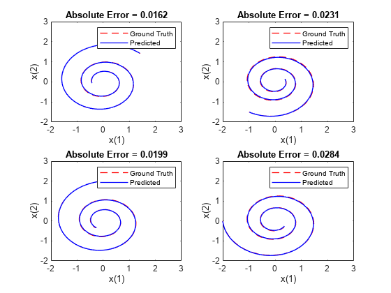
Visualize Predictions
Visualize the predicted solutions for different initial conditions against the ground truth solutions with the function plotTrueAndPredictedSolutions, listed in the Plot True and Predicted Solutions Function section of the example.
figure
subplot(2,2,1)
plotTrueAndPredictedSolutions(xTrue1, xPred1);
subplot(2,2,2)
plotTrueAndPredictedSolutions(xTrue2, xPred2);
subplot(2,2,3)
plotTrueAndPredictedSolutions(xTrue3, xPred3);
subplot(2,2,4)
plotTrueAndPredictedSolutions(xTrue4, xPred4);
Helper Functions
Model Function
The model function, which defines the neural network used to make predictions, is composed of a single neural ODE call. For each observation, this function takes a vector of length stateSize, which is used as initial condition for solving numerically the ODE with the function odeModel, which represents the learnable right-hand side of the ODE to be solved, as right hand side and a vector of time points tspan defining the time at which the numerical solution is output. The function uses the vector tspan for each observation, regardless of the initial condition, since the learned system is autonomous. That is, the odeModel function does not explicitly depend on time.
function X = model(tspan,X0,neuralOdeParameters)

X = dlode45(@odeModel,tspan,X0,neuralOdeParameters,DataFormat="CB");

end
ODE Model
The odeModel function is the learnable right-hand side used in the call to dlode45. It takes as input a vector of size stateSize, enlarges it so that it has length hiddenSize, and applies a nonlinearity function tanh. Then the function compresses the vector again to have length stateSize.
function y = odeModel(~,y,theta)

y = tanh(theta.fc1.Weights*y + theta.fc1.Bias);
y = theta.fc2.Weights*y + theta.fc2.Bias;

end
Model Loss Function
This function takes as inputs a vector tspan, a set of initial conditions X0, the learnable parameters neuralOdeParameters, and target sequences targets. It computes the predictions with the model function, and compares them with the given targets sequences. Finally, it computes the loss and the gradient of the loss with respect to the learnable parameters of the neural ODE.
function [loss,gradients] = modelLoss(tspan,X0,neuralOdeParameters,targets)

% Compute predictions.
X = model(tspan,X0,neuralOdeParameters);

% Compute L1 loss.
loss = l1loss(X,targets,NormalizationFactor="all-elements",DataFormat="CBT");

% Compute gradients.
gradients = dlgradient(loss,neuralOdeParameters);

end
Create Mini-Batches Function
The createMiniBatch function creates a batch of observations of the target dynamics. It takes as input the total number of time steps of the ground truth data numTimesteps, the number of consecutive time steps to be returned for each observation numTimesPerObs, the number of observations miniBatchSize, and the ground truth data X.
function [x0, targets] = createMiniBatch(numTimesteps,numTimesPerObs,miniBatchSize,X)

% Create batches of trajectories.
s = randperm(numTimesteps - numTimesPerObs, miniBatchSize);

x0 = dlarray(X(:, s));
targets = zeros([size(X,1) miniBatchSize numTimesPerObs]);

for i = 1:miniBatchSize
    targets(:, i, 1:numTimesPerObs) = X(:, s(i) + 1:(s(i) + numTimesPerObs));
end

end
Plot True and Predicted Solutions Function
The plotTrueAndPredictedSolutions function takes as input the true solution xTrue, the approximated solution xPred computed with the learned neural ODE model, and the corresponding initial condition x0Str. It computes the error between the true and predicted solutions and plots it in a phase diagram.
function plotTrueAndPredictedSolutions(xTrue,xPred)

xPred = squeeze(xPred)';

err = mean(abs(xTrue(2:end,:) - xPred), "all");

plot(xTrue(:,1),xTrue(:,2),"r--",xPred(:,1),xPred(:,2),"b-",LineWidth=1)

title("Absolute Error = " + num2str(err,"%.4f"))
xlabel("x(1)")
ylabel("x(2)")

xlim([-2 3])
ylim([-2 3])

legend("Ground Truth","Predicted")

end
[1] Chen, Ricky T. Q., Yulia Rubanova, Jesse Bettencourt, and David Duvenaud. “Neural Ordinary Differential Equations.” Preprint, submitted December 13, 2019. https://arxiv.org/abs/1806.07366.
[2] Shampine, Lawrence F., and Mark W. Reichelt. “The MATLAB ODE Suite.” SIAM Journal on Scientific Computing 18, no. 1 (January 1997): 1–22. https://doi.org/10.1137/S1064827594276424.
See Also
dlode45 | dlarray | dlgradient | dlfeval | adamupdate
Topics
- Custom Loss Functions
- Custom Training Loops
- Custom Training Loop Model Loss Functions
- Train Neural ODE Network
- Train Latent ODE Network with Irregularly Sampled Time-Series Data
- Train Neural ODE Network with Control Input
- Specify Training Options in Custom Training Loop
- Train Network Using Custom Training Loop
- List of Functions with dlarray Support