Explore Semantic Segmentation Network Using Grad-CAM
This example shows how to explore the predictions of a pretrained semantic segmentation network using Grad-CAM.
A semantic segmentation network classifies every pixel in an image, resulting in an image that is segmented by class. You can use Grad-CAM, a deep learning visualization technique, to see which regions of the image are important for the pixel classification decision.
Download Pretrained Network
Download a semantic segmentation network trained on the CamVid data set [1] from the University of Cambridge. For more information on building and training a semantic segmentation network, see Semantic Segmentation Using Deep Learning (Computer Vision Toolbox).
pretrainedURL = "https://ssd.mathworks.com/supportfiles/vision/data/deeplabv3plusResnet18CamVid_v2.zip";
pretrainedFolder = fullfile(tempdir,"pretrainedNetwork");
pretrainedNetworkZip = fullfile(pretrainedFolder,"deeplabv3plusResnet18CamVid_v2.zip");
if ~exist(pretrainedNetworkZip,'file')
    mkdir(pretrainedFolder);
disp("Downloading pretrained network (58 MB)...");
    websave(pretrainedNetworkZip,pretrainedURL);
end
unzip(pretrainedNetworkZip, pretrainedFolder)
Load the pretrained network.
pretrainedNetwork = fullfile(pretrainedFolder,"deeplabv3plusResnet18CamVid_v2.mat");
pretrainedNet = load(pretrainedNetwork,"net");
net = pretrainedNet.net;
Perform Semantic Segmentation
Before analyzing the network predictions using Grad-CAM, use the pretrained network to segment a test image.
Load a test image and resize it to match the size required by the network.
img = imread("parkinglot_left.png");
inputSize = net.Layers(1).InputSize(1:2);
img = imresize(img,inputSize);
Use the semanticseg function to predict the pixel labels of the image.
predLabels = semanticseg(img,net);
Overlay the segmentation results on the original image and display the results.
cmap = camvidColorMap;
segImg = labeloverlay(img,predLabels,Colormap=cmap,Transparency=0.4);

figure
imshow(segImg)
classes = camvidClasses();
pixelLabelColorbar(cmap,classes)
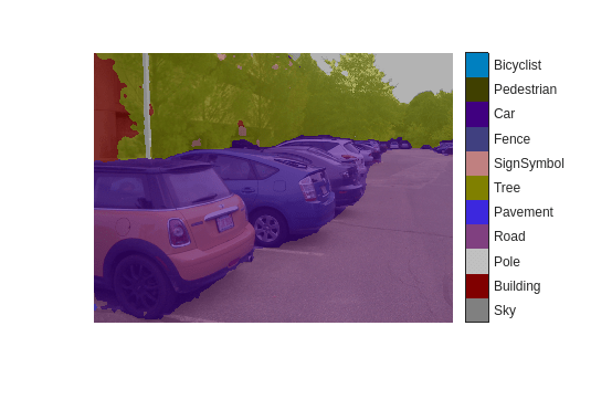
The network does misclassify some areas, for example, the road near the tires is misclassified as car. Next, you will explore the network predictions with Grad-CAM to gain insight into why the network misclassified certain regions.
Explore Network Predictions
Deep networks are complex, so understanding how a network determines a particular prediction is difficult. You can use Grad-CAM to see which areas of the test image the semantic segmentation network is using to make its pixel classifications.
Grad-CAM computes the gradient of a differentiable output, such as class score, with respect to the convolutional features in a chosen layer. Grad-CAM is typically used for image classification tasks [2]; however, it can also be extended to semantic segmentation problems [3].
In semantic segmentation tasks, the softmax layer of the network outputs a score for each class for every pixel in the original image. This contrasts with standard image classification problems, where the softmax layer outputs a score for each class for the entire image. The Grad-CAM map for class is
where
is the number of pixels, is the feature map of interest, and corresponds to a scalar class score. For a simple image classification problem, is the softmax score for the class of interest. For semantic segmentation, you can obtain by reducing the pixel-wise class scores for the class of interest to a scalar. For example, sum over the spatial dimensions of the softmax layer: , where is the pixels in the softmax layer of a semantic segmentation network [3]. The map highlights areas that influence the decision for class . Higher values indicate regions of the image that are important for the pixel classification decision.
To use Grad-CAM, you must select a feature layer to extract the feature map from and a reduction layer to extract the output activations from. Use analyzeNetwork to find the layers to use with Grad-CAM.
analyzeNetwork(net)
Specify a feature layer. Typically this is a ReLU layer which takes the output of a convolutional layer at the end of the network.
featureLayer = "dec_relu4";Specify a reduction layer. The gradCAM function sums the spatial dimensions of the reduction layer, for the specified classes, to produce a scalar value. This scalar value is then differentiated with respect to each feature in the feature layer. For semantic segmentation problems, the reduction layer is usually the softmax layer.
reductionLayer = "softmax-out";Compute the Grad-CAM map for the road and pavement classes. Classes 4 and 9 correspond to the "Road" and "Car" classes, respectively.
classNames = [4 9];

gradCAMMap = gradCAM(net,img,classNames, ...
    ReductionLayer=reductionLayer, ...
    FeatureLayer=featureLayer);
Compare the Grad-CAM map for the two classes to pixel labels predicted by the network.
figure
subplot(2,2,1)
imshow(img)
title("Test Image")
subplot(2,2,2)
imshow(segImg)
title("Semantic Segmentation")
subplot(2,2,3)
imshow(img)
hold on
imagesc(gradCAMMap(:,:,1),AlphaData=0.5)
title("Grad-CAM: " + classes(classNames(1)))
colormap jet
subplot(2,2,4)
imshow(img)
hold on
imagesc(gradCAMMap(:,:,2),AlphaData=0.5)
title("Grad-CAM: " + classes(classNames(2)))
colormap jet
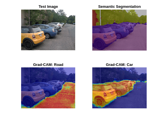
The Grad-CAM maps and semantic segmentation map show similar highlighting. The Grad-CAM map for the road class shows a fairly even distribution of importance for the classification decision of the network. For the car class, the center mass of each car is of most importance as we can expect. The network possibly misclassifies road areas near the bottom of the cars because of the poor resolution between the tire and road boundary, as well as shadows of the cars blurring their boundary with the road.
Explore Intermediate Layers
The Grad-CAM map resembles the semantic segmentation map when you use a layer near the end of the network for the computation. You can also use Grad-CAM to investigate intermediate layers in the trained network. Earlier layers have a small receptive field size and learn small, low-level features compared to the layers at the end of the network.
Compute the Grad-CAM map for layers that are successively deeper in the network.
layers = ["res5b_relu","catAspp","dec_relu1"];
numLayers = length(layers);
The res5b_relu layer is near the middle of the network, whereas dec_relu1 is near the end of the network.
Investigate the network classification decisions for the car and road classes. For each layer and class, compute the Grad-CAM map.
numClasses = length(classNames);

gradCAMMaps = [];
for i = 1:numLayers
    gradCAMMaps(:,:,:,i) = gradCAM(net,img,classNames, ...
        ReductionLayer=reductionLayer, ...
        FeatureLayer=layers(i));
end
Display the Grad-CAM maps for each layer and each class. The rows represent the map for each layer, with the layers ordered from those early in the network to those at the end of the network.
figure;
idx = 1;
for i=1:numLayers
    for j=1:numClasses
subplot(numLayers,numClasses,idx)
        imshow(img)
        hold on
        imagesc(gradCAMMaps(:,:,j,i),AlphaData=0.5)
        title(sprintf("%s (%s)",classes(classNames(j)),layers(i)), ...
            Interpreter="none")
        colormap jet
        idx = idx + 1;
    end
end
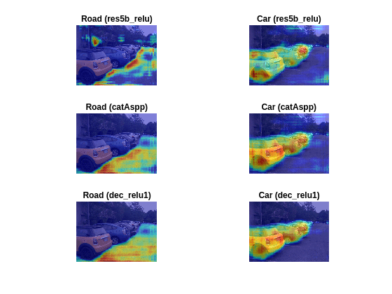
The later layers produce maps very similar to the segmentation map. However, the layers earlier in the network produce more abstract results and are typically more concerned with lower level features like edges, with less awareness of semantic classes. For example, in the maps for earlier layers, you can see that for both car and road classes, the sky is highlighted. This suggests that the earlier layers focus on areas of the image that are related to the class but do not necessarily belong to it.
Supporting Functions
function classes = camvidClasses()
% Return the CamVid class names used during network training.
%
% The CamVid data set has 32 classes. Group them into 11 classes following
% the original SegNet training methodology [1].
%
% The 11 classes are:
%   "Sky", "Building", "Pole", "Road", "Pavement", "Tree", "SignSymbol",
%   "Fence", "Car", "Pedestrian",  and "Bicyclist".
%
classes = [
    "Sky"
    "Building"
    "Pole"
    "Road"
    "Pavement"
    "Tree"
    "SignSymbol"
    "Fence"
    "Car"
    "Pedestrian"
    "Bicyclist"
    ];
end
function pixelLabelColorbar(cmap, classNames)
% Add a colorbar to the current axis. The colorbar is formatted
% to display the class names with the color.

colormap(gca,cmap)

% Add a colorbar to the current figure.
c = colorbar("peer",gca);

% Use class names for tick marks.
c.TickLabels = classNames;
numClasses = size(cmap,1);

% Center tick labels.
c.Ticks = 1/(numClasses*2):1/numClasses:1;

% Remove tick marks.
c.TickLength = 0;
end
function cmap = camvidColorMap
% Define the colormap used by the CamVid data set.

cmap = [
    128 128 128   % Sky
    128 0 0       % Building
    192 192 192   % Pole
    128 64 128    % Road
    60 40 222     % Pavement
    128 128 0     % Tree
    192 128 128   % SignSymbol
    64 64 128     % Fence
    64 0 128      % Car
    64 64 0       % Pedestrian
    0 128 192     % Bicyclist
    ];

% Normalize between [0 1].
cmap = cmap ./ 255;
end
References
[1] Brostow, Gabriel J., Julien Fauqueur, and Roberto Cipolla. “Semantic Object Classes in Video: A High-Definition Ground Truth Database.” Pattern Recognition Letters 30, no. 2 (January 2009): 88–97. https://doi.org/10.1016/j.patrec.2008.04.005.
[2] Selvaraju, R. R., M. Cogswell, A. Das, R. Vedantam, D. Parikh, and D. Batra. "Grad-CAM: Visual Explanations from Deep Networks via Gradient-Based Localization." In IEEE International Conference on Computer Vision (ICCV), 2017, pp. 618–626. Available at Grad-CAM on the Computer Vision Foundation Open Access website.
[3] Vinogradova, Kira, Alexandr Dibrov, and Gene Myers. “Towards Interpretable Semantic Segmentation via Gradient-Weighted Class Activation Mapping (Student Abstract).” Proceedings of the AAAI Conference on Artificial Intelligence 34, no. 10 (April 3, 2020): 13943–44. https://doi.org/10.1609/aaai.v34i10.7244.
See Also
gradCAM | semanticseg (Computer Vision Toolbox) | pixelLabelDatastore (Computer Vision Toolbox)