Prepare Network for Transfer Learning Using Deep Network Designer

This example shows how to prepare a network for transfer learning interactively using the Deep Network Designer app.

Transfer learning is the process of taking a pretrained deep learning network and fine-tuning it to learn a new task. Using transfer learning is usually faster and easier than training a network from scratch. You can quickly transfer learned features to a new task using a smaller amount of data.

Extract Data

Extract the MathWorks Merch dataset. This is a small dataset containing 75 images of MathWorks merchandise, belonging to five different classes (cap, cube, playing cards, screwdriver, and torch). The data is arranged such that the images are in subfolders that correspond to these five classes.

folderName = "MerchData";
unzip("MerchData.zip",folderName);

Create an image datastore. An image datastore enables you to store large collections of image data, including data that does not fit in memory, and efficiently read batches of images during training of a neural network. Specify the folder with the extracted images and indicate that the subfolder names correspond to the image labels.

imds = imageDatastore(folderName, ...
    IncludeSubfolders=true, ...
    LabelSource="foldernames");

Display some sample images.

numImages = numel(imds.Labels);
idx = randperm(numImages,16);
I = imtile(imds,Frames=idx);
figure
imshow(I)

Extract the class names and the number of classes.

classNames = categories(imds.Labels);
numClasses = numel(classNames)

numClasses = 
5

Partition the data into training, validation, and testing datasets. Use 70% of the images for training, 15% for validation, and 15% for testing. The splitEachLabel function splits the image datastore into two new datastores.

[imdsTrain,imdsValidation,imdsTest] = splitEachLabel(imds,0.7,0.15,0.15,"randomized");

Select a Pretrained Network

To open Deep Network Designer, on the Apps tab, under Machine Learning and Deep Learning, click the app icon. Alternatively, you can open the app from the command line:

deepNetworkDesigner

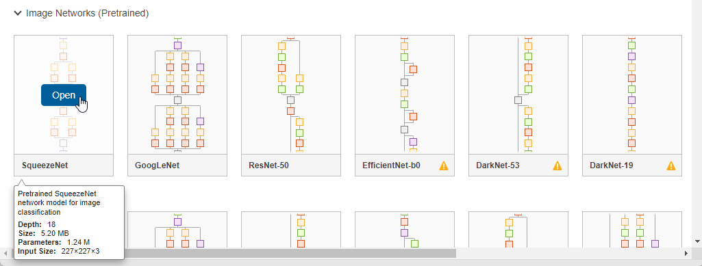
Deep Network Designer provides a selection of pretrained image classification networks that have learned rich feature representations suitable for a wide range of images. Transfer learning works best if your images are similar to the images originally used to train the network. If your training images are natural images like those in the ImageNet database, then any of the pretrained networks is suitable. For a list of available networks and how to compare them, see Pretrained Deep Neural Networks.

If your data is very different from the ImageNet data—for example, if you have tiny images, spectrograms, or nonimage data—training a new network might be better. For an example showing how to train a network from scratch, see Get Started with Time Series Forecasting.

SqueezeNet does not require an additional support package. For other pretrained networks, if you do not have the required support package installed, then the app provides the Install option.

Select SqueezeNet from the list of pretrained networks and click Open.

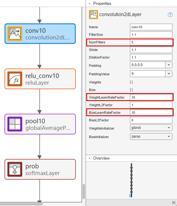
To prepare the network for transfer learning:

• Set the Number of classes to the new number of classes — in this example, 5. This sets the NumFilters property in the last learnable layer 'conv10'. The NumFilters property defines the number of classes for classification problems.

• Set the Learning rate in the last learnable layer to 10 so that learning is faster in the last learnable layer than in the transferred layers. This sets the WeightLearnRateFactor and BiasLearnRateFactor properties of the last learnable layer to 10.

• Click Import.

Before R2025b: To adapt the network to the new data, you must click the last learnable layer in Designer pane, click Unlock Layer, set its NumFilters property to the number of classes in the new data, and increase its WeightLearnRateFactor and BiasLearnRateFactor properties.

Explore Network

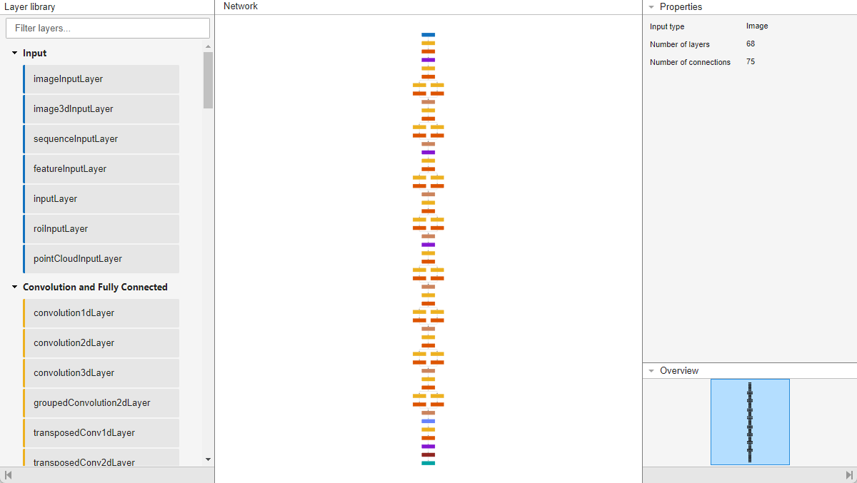
Deep Network Designer displays a zoomed-out view of the whole network in the Designer pane.

Explore the network plot. To zoom in with the mouse, use Ctrl+scroll wheel. To pan, use the arrow keys, or hold down the scroll wheel and drag the mouse. Select a layer to view its properties. Deselect all layers to view the network summary in the Properties pane.

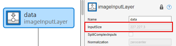
Select the image input layer, 'data'. You can see that the input size for this network is 227-by-227-by-3 pixels.

Save the input size in the variable inputSize.

inputSize = [227 227 3];

Check Network

To check that the network is ready for training, click Analyze. The Deep Learning Network Analyzer reports zero errors or warnings, therefore, the network is ready for training.

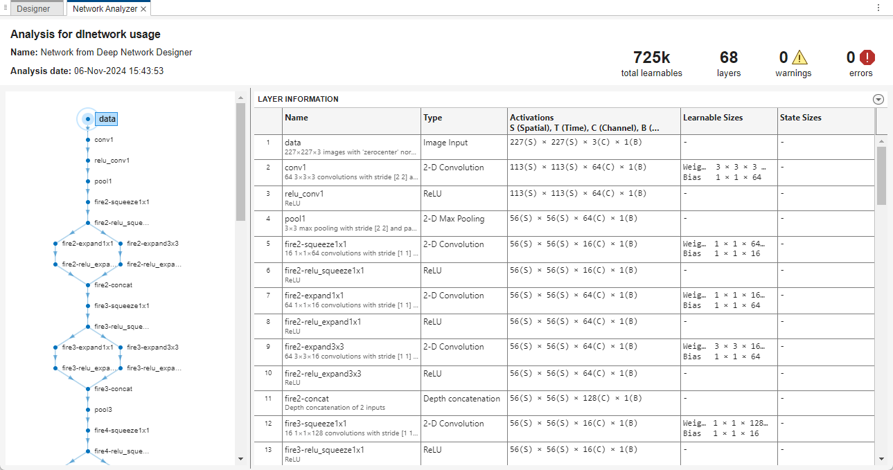
To export the network, click Export and then click OK. The app saves the network in the variable net_1.

Prepare Data for Training

The images in the datastore can have different sizes. To automatically resize the training images, use an augmented image datastore. Data augmentation also helps prevent the network from overfitting and memorizing the exact details of the training images. Specify these additional augmentation operations to perform on the training images: randomly flip the training images along the vertical axis, and randomly translate them up to 30 pixels horizontally and vertically.

pixelRange = [-30 30];

imageAugmenter = imageDataAugmenter( ...
    RandXReflection=true, ...
    RandXTranslation=pixelRange, ...
    RandYTranslation=pixelRange);

augimdsTrain = augmentedImageDatastore(inputSize(1:2),imdsTrain, ...
    DataAugmentation=imageAugmenter);

To automatically resize the validation and testing images without performing further data augmentation, use an augmented image datastore without specifying any additional preprocessing operations.

augimdsValidation = augmentedImageDatastore(inputSize(1:2),imdsValidation);
augimdsTest = augmentedImageDatastore(inputSize(1:2),imdsTest);

Specify Training Options

Specify the training options. Choosing among the options requires empirical analysis. To explore different training option configurations by running experiments, you can use the Experiment Manager app.

• Train using the Adam optimizer.

• Set the initial learn rate to a small value to slow down learning in the transferred layers.

• Specify a small number of epochs. An epoch is a full training cycle on the entire training data set. For transfer learning, you do not need to train for as many epochs.

• Specify validation data and a validation frequency so that the accuracy on the validation data is calculated once every epoch.

• Specify the mini-batch size, that is, how many images to use in each iteration. To ensure the whole data set is used during each epoch, set the mini-batch size to evenly divide the number of training samples.

• Display the training progress in a plot and monitor the accuracy metric.

• Disable the verbose output.

options = trainingOptions("adam", ...
    InitialLearnRate=0.0001, ...
    MaxEpochs=8, ...
    ValidationData=imdsValidation, ...
    ValidationFrequency=5, ...
    MiniBatchSize=11, ...
    Plots="training-progress", ...
    Metrics="accuracy", ...
    Verbose=false);

Train Neural Network

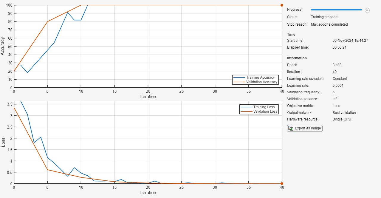
Train the neural network using the trainnet function. For classification tasks, use cross-entropy loss. By default, the trainnet function uses a GPU if one is available. Using a GPU requires a Parallel Computing Toolbox™ license and a supported GPU device. For information on supported devices, see GPU Computing Requirements (Parallel Computing Toolbox). Otherwise, the trainnet function uses the CPU. To specify the execution environment, use the ExecutionEnvironment training option.

net = trainnet(imdsTrain,net_1,"crossentropy",options);

Test Neural Network

Classify the test images. To make predictions with multiple observations, use the minibatchpredict function. To convert the prediction scores to labels, use the scores2label function. The minibatchpredict function automatically uses a GPU if one is available.

YTest = minibatchpredict(net,augimdsTest);
YTest = scores2label(YTest,classNames);

Visualize the classification accuracy in a confusion chart.

TTest = imdsTest.Labels;
figure
confusionchart(TTest,YTest);

Make Predictions with New Data

Classify an image. Read an image from a JPEG file, resize it, and convert to the single data type.

im = imread("MerchDataTest.jpg");
im = imresize(im,inputSize(1:2));
X = single(im);

Classify the image. To make prediction with a single observation, use the predict function. To use a GPU, first convert the data to gpuArray.

if canUseGPU
    X = gpuArray(X);
end
scores = predict(net,X);
[label,score] = scores2label(scores,classNames);

Display the image with the predicted label and the corresponding score.

figure
imshow(im)
title(string(label) + " (Score: " + score + ")")