Discrete Transfer Function Estimator
Compute estimate of frequency-domain transfer function of system
Libraries:
DSP System Toolbox /
Estimation /
Power Spectrum Estimation
Description
The Discrete Transfer Function Estimator block estimates the frequency-domain transfer function of a system using the Welch’s method of averaged modified periodograms.
The block buffers the input data into overlapping segments. You can set the length of the data segment and the amount of data overlap through the parameters set in the block dialog box. The sample rate of the block is equal to 1/T. T is the sample time of the inputs to the block.
The block first applies a window function to the two inputs, x and y, and then scales them by the window power. It takes the FFT of each signal, calling them X and Y. The block calculates Pxx which is the square magnitude of the FFT, X. The block then calculates Pyx which is X multiplied by the conjugate of Y. The output transfer function estimate, H, is calculated by dividing Pyx by Pxx.
Examples
Estimate Frequency-Domain Transfer Function of System Using Random Excitation Input
This example shows how to use the Discrete Transfer Function Estimator block to estimate the frequency-domain transfer function of a system.
Open the ex_discretetransferfunctionestimator.slx
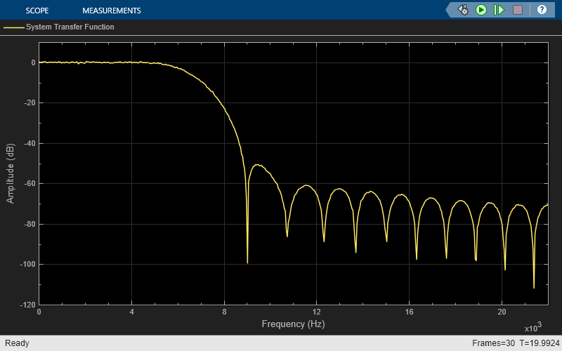
model. The Random Source block generates the system input signal that you pass through the x port of the Discrete Transfer Function Estimator block. The sample rate of the input signal is 44.1 KHz. This input signal passes through a lowpass filter with a normalized cutoff frequency of 0.3. The filtered signal represents the system output signal that you input through the port y of the Discrete Transfer Function Estimator block. Because the Discrete Transfer Function Estimator block outputs complex values, compute the magnitude of the output signal to generate a plot of the transfer function estimate.
Run the model. The array plot shows the system transfer function, a lowpass filter that matches the frequency response of the Discrete FIR Filter block.
Ports
Input
x — System input signal
vector | matrix
Specify the system input signal as a vector or a matrix.
The inputs x and y must have the same size and data type.
Data Types: double
| single
y — System output signal
vector | matrix
Specify the system output signal as a vector or a matrix.
The inputs x and y must have the same size and data type.
Data Types: double
| single
Output
Output — Transfer function estimate
vector | matrix
Transfer function estimate, returned as a vector or a matrix. For more details on how the block computes the transfer function estimate, see Algorithms.
Data Types: double
| single
Parameters
Window length source — Window length source
Same as input frame
length
(default) | Specify on dialog
Specify the source of the window length value. You can set this parameter to:
Same as input frame length
— Window length is set to the frame size of the input.Specify on dialog
— Window length is the value you specify in Window length.
Window length — Window length
1024
(default) | positive integer ≥ 2
Specify the length of the window, in samples, used to compute the spectrum
estimate as a positive integer greater than or equal to
2
.
Dependencies
To enable this parameter, set Window length
source to Specify on
dialog
.
Window overlap (%) — Percentage of overlap between windows
0
(default) | nonnegative scalar
Specify the percentage of overlap between successive data windows as a
nonnegative scalar in the range
[0
,100
).
Averaging method — Averaging method
Running
(default) | Exponential
Specify the averaging method as Running
or
Exponential
. In the running averaging method,
the block computes an equally weighted average of specified number of
spectrum estimates defined by Number of spectral
averages parameter. In the exponential method, the block
computes the average over samples weighted by an exponentially decaying
forgetting factor.
Specify forgetting factor from input port — Specify forgetting factor from input port
off
(default) | on
Select this check box to specify the forgetting factor from an input port. When you do not select this check box, the forgetting factor is specified through the Forgetting factor parameter.
Dependencies
To enable this parameter, set Averaging method to
Exponential
.
Forgetting factor — Forgetting factor
0.9
(default) | positive scalar ≤ 1
Specify the exponential weighting forgetting factor as a positive scalar ≤
1
.
Dependencies
To enable this parameter, set Averaging method to
Exponential
and clear the
Specify forgetting factor from input port
parameter.
Number of spectral averages — Number of spectral averages
1
(default) | positive integer
Specify the number of spectral averages as a positive integer. The Transfer Function Estimator block computes the current estimate by averaging the last N estimates. N is the number of spectral averages.
Dependencies
To enable this parameter, set Averaging method to
Running
.
FFT length source — Source of FFT length value
Auto
(default) | Property
Specify the source of the FFT length value as
Auto
or Property
.
When the source of the FFT length is set to
Auto
, the block sets the FFT length to the
input frame size. When the source of the FFT length is set to
Property
, you specify the FFT length in the
FFT length parameter.
FFT length — FFT length
128
(default) | positive integer
Specify the length of the FFT that the Discrete Transfer Function Estimator block uses to compute spectral estimates as a positive integer.
Window function — Window function
Hann
(default) | Chebyshev
| Flat Top
| Hamming
| Kaiser
| Rectangular
Specify a window function for the Discrete Transfer Function Estimator block. Possible values are:
Hann
Chebyshev
Flat Top
Hamming
Kaiser
Rectangular
Sidelobe attenuation of window (dB) — Sidelobe attenuation of window
60
(default) | positive scalar
Specify the sidelobe attenuation of the window as a positive scalar in dB.
Dependencies
To enable this parameter, set Window function to
Kaiser
or
Chebyshev
.
Frequency range — Frequency range of the transfer function estimate
Centered
(default) | One-sided
| Two-sided
Specify the frequency range of the transfer function estimate.
Centered
–– The block computes the centered two-sided transfer function of the real or complex input signals, x and y.onesided
–– The block computes the one-sided transfer function of real input signals, x and y.twosided
–– The block computes the two-sided transfer function of the real or complex input signals, x and y.
Output magnitude squared coherence estimate — Magnitude squared coherence estimate
off
(default) | on
Select this check box to compute and output the magnitude squared coherence estimate using Welch’s averaged, modified periodogram method. The magnitude squared coherence estimate indicates how well two inputs correspond to each other at each frequency.
Simulate using — Type of simulation to run
Interpreted execution
(default) | Code generation
Specify the type of simulation to run. You can set this parameter to:
Interpreted execution
–– Simulate model using the MATLAB® interpreter. This option shortens startup time.Code generation
–– Simulate model using generated C code. The first time you run a simulation, Simulink® generates C code for the block. The C code is reused for subsequent simulations as long as the model does not change. This option requires additional startup time but provides faster subsequent simulations.
Block Characteristics
Data Types |
|
Multidimensional Signals |
|
Variable-Size Signals |
|
Algorithms
Welch's Method of Averaged Modified Periodograms
Give two signal inputs, x and y:
Multiply the inputs by the window and scale the result by the window power.
Take FFT of the signals, X and Y.
Compute the current power spectral density estimates, Pxx, Pyy, and the current cross power spectral density estimate, Pyx, by taking the moving average of last N number of Z1, Z2, and Z3 vectors, respectively:
Z1 = X.*conj(X)
Z2 = Y.*conj(Y)
Z3 = Y.*conj(X)
For details on the moving average methods, see Averaging Method.
The transfer function estimate is calculated by dividing
Pyx
by
Pxx
.
The magnitude squared coherence, Cxy
, is
defined by the following equation:
Extended Capabilities
C/C++ Code Generation
Generate C and C++ code using Simulink® Coder™.
Version History
Introduced in R2014aR2024a: Change in the default value of Simulate using parameter
The default value of the Simulate using parameter is now
Interpreted execution
. With this change, the block uses the
MATLAB interpreter for simulation by default.
MATLAB Command
You clicked a link that corresponds to this MATLAB command:
Run the command by entering it in the MATLAB Command Window. Web browsers do not support MATLAB commands.
Select a Web Site
Choose a web site to get translated content where available and see local events and offers. Based on your location, we recommend that you select: .
You can also select a web site from the following list:
How to Get Best Site Performance
Select the China site (in Chinese or English) for best site performance. Other MathWorks country sites are not optimized for visits from your location.
Americas
- América Latina (Español)
- Canada (English)
- United States (English)
Europe
- Belgium (English)
- Denmark (English)
- Deutschland (Deutsch)
- España (Español)
- Finland (English)
- France (Français)
- Ireland (English)
- Italia (Italiano)
- Luxembourg (English)
- Netherlands (English)
- Norway (English)
- Österreich (Deutsch)
- Portugal (English)
- Sweden (English)
- Switzerland
- United Kingdom (English)