Compress Deep DOA Estimation Network Using Pruning and Projection
R2026bThis example shows how to compress the deep learning network trained in the Deploy Direction of Arrival Estimation Using Deep Learning on Desktop example for direction-of-arrival (DOA) estimation using structured pruning and projection techniques. These compression methods reduce the network size and inference time while maintaining estimation accuracy. This characteristic enables efficient real-time deployment on resource-constrained hardware.
Compression Workflow
The compression pipeline consists of two stages applied sequentially:
Structured pruning − Remove entire convolution filters ranked by first-order Taylor importance scores, then fine-tune to recover accuracy.
Projection − Apply PCA to layer activations and replace convolution and fully connected layers with lower-rank equivalents.
Together, these stages significantly reduce parameter count, memory footprint, and inference time while preserving DOA estimation accuracy.
Load Trained Network and Training Data
Load the pretrained deep DOA estimator network.
if exist("deepDOAEstimator.mat","file") ~= 2
    zipFile = matlab.internal.examples.downloadSupportFile("dsp","DeepDOAEstimator.zip");
    unzip(zipFile,cd)
end
file = load("deepDOAEstimator.mat");
deepDOAEstimator = file.deepDOAEstimator;
Generate the training data set using Phased Array System Toolbox simulations. The data set consists of covariance matrices derived from signals received at an 8-element uniform linear array (ULA) under multiple SNR scenarios.
dataset = helperGenerateTrainData;
Analyze Original Network
The network consists of three convolutional blocks (each with batch normalization and ReLU activation), followed by two fully connected layers with dropout, and a sigmoid output layer producing a 181-element probability vector over the angle grid from −90° to 90°. Examine the parameter count and memory footprint.
originalMetrics = estimateNetworkMetrics(deepDOAEstimator);
originalLearnables = sum(originalMetrics.NumberOfLearnables);
originalMemory = sum(originalMetrics.("ParameterMemory (MB)"));
fprintf("Original network: %d learnables, %.4f MB\n", ...
    originalLearnables, originalMemory)
Original network: 2309621 learnables, 8.8105 MB
Step 1: Structured Pruning
Structured pruning removes entire convolution filters that contribute least to the network output. This example uses Taylor-score-based pruning, which involves these steps:
Compute the gradient of the loss with respect to activations and filter weights.
Compute first-order Taylor scores to estimate each filter's importance.
Rank filters based on the obtained scores.
Remove the lowest-impact filters (pruning step).
Fine-tune the pruned network.
Repeat for multiple iterations.
Define the pruning parameters.
maxPruningIterations = 5;
maxToPrune = 8;
learnRate = 1e-5;
momentum = 0.9;
miniBatchSize = 256;
numMinibatchUpdates = 100;
Create mini-batch queues for training.
dsXTrain = arrayDatastore(dataset.trainData, IterationDimension=4);
dsYTrain = arrayDatastore(dlarray(extractdata(dataset.trainLabels)), IterationDimension=2);
dsTrain = combine(dsXTrain, dsYTrain);
mbqTrain = minibatchqueue(dsTrain, ...
    MiniBatchSize=miniBatchSize, ...
    PartialMiniBatch="return", ...
    MiniBatchFormat=["SSCUB","CB"]);
You can skip pruning by using the prepruned network. To prune the network as the example runs, set pruneNow to true. To skip pruning and use the prepruned network, set pruneNow to false.
pruneNow =false; if pruneNow prunableNet = taylorPrunableNetwork(deepDOAEstimator); maxPrunableFilters = prunableNet.NumPrunables; figure(Position=[10 10 700 500]) tl = tiledlayout(2,1); lossAx = nexttile; lineLossFinetune = animatedline(Color=[0.85 0.325 0.098]); ylim([0 inf]) xlabel("Fine-Tuning Iteration") ylabel("Loss") grid on title("Mini-Batch Loss During Pruning") xTickPos = []; numPrunablesAx = nexttile; lineNumPrunables = animatedline(Color=[0.4660 0.6740 0.1880], ... LineWidth=2, Marker="^"); ylim([80 160]) xlabel("Pruning Iteration") ylabel("Prunable Filters") grid on addpoints(lineNumPrunables, 0, maxPrunableFilters) title("Number of Prunable Convolution Filters After Pruning") start = tic; iteration = 0; for pruningIteration = 1:maxPruningIterations shuffle(mbqTrain); velocity = []; fineTuningIteration = 0; while hasdata(mbqTrain) iteration = iteration + 1; fineTuningIteration = fineTuningIteration + 1; [X, T] = next(mbqTrain); [loss, pruningActivations, pruningGradients, netGradients, state] = ... dlfeval(@modelLossPruning, prunableNet, X, T); prunableNet.State = state; [prunableNet, velocity] = sgdmupdate(prunableNet, ... netGradients, velocity, learnRate, momentum); prunableNet = updateScore(prunableNet, ... pruningActivations, pruningGradients); D = duration(0,0,toc(start),Format="hh:mm:ss"); addpoints(lineLossFinetune, iteration, loss) title(tl, "Pruning Iteration: " + pruningIteration + ... " of " + maxPruningIterations + ... ", Elapsed: " + string(D)) xlim(numPrunablesAx, lossAx.XLim) drawnow if fineTuningIteration > numMinibatchUpdates break end end prunableNet = updatePrunables(prunableNet, MaxToPrune=maxToPrune); addpoints(lineNumPrunables, iteration, prunableNet.NumPrunables) xTickPos = [xTickPos, iteration]; xticks(lossAx, xTickPos) xticks(numPrunablesAx, [0, xTickPos]) xticklabels(numPrunablesAx, ["Unpruned", string(1:pruningIteration)]) drawnow end prunedNet = dlnetwork(prunableNet); else if exist("compressedDOANetworks.mat","file") ~= 2 %#ok<*UNRCH> zipFile=matlab.internal.examples.downloadSupportFile("DSP/data","DeepDOAEstimatorCompressed.zip"); unzip(zipFile,tempdir) movefile(fullfile(tempdir, "DeepDOAEstimatorCompressed", "compressedDOANetworks.mat"), cd); end savedNetworks = load("compressedDOANetworks.mat"); prunedNet = savedNetworks.prunedNet; end
Retrain Network After Pruning
Pruning structurally changes the network, which temporarily increases loss and reduces accuracy. Retrain the network for a few epochs to recover performance.
if pruneNow
    metric = accuracyMetric(ClassificationMode="multilabel");

    options = trainingOptions("adam", ...
        InitialLearnRate=1e-4, ...
        MaxEpochs=7, ...
        MiniBatchSize=256, ...
        Shuffle="every-epoch", ...
        Verbose=false, ...
        Plots="training-progress", ...
        ExecutionEnvironment="auto", ...
        Metrics=metric, ...
        OutputNetwork="last-iteration");

    prunedNet = trainnet(dataset.trainData, dataset.trainLabels, ...
        prunedNet, @(y,t)customLoss(y,t), options);
end
Analyze the pruned network metrics.
prunedMetrics = estimateNetworkMetrics(prunedNet);
prunedLearnables = sum(prunedMetrics.NumberOfLearnables);
prunedMemory = sum(prunedMetrics.("ParameterMemory (MB)"));
fprintf("Pruned network: %d learnables, %.4f MB\n", ...
    prunedLearnables, prunedMemory)
Pruned network: 1903931 learnables, 7.2629 MB
fprintf("Reduction: %.1f%% fewer learnables, %.1f%% less memory\n", ...
    100*(1 - prunedLearnables/originalLearnables), ...
    100*(1 - prunedMemory/originalMemory))
Reduction: 17.6% fewer learnables, 17.6% less memory
Pruning reduces the number of convolutional filters in the network from 192 to 152, yielding approximately 17% fewer learnable parameters overall.
Step 2: Projection
Projection compresses network layers by applying principal component analysis (PCA) to neuron activations. This technique re-expresses the learned weights using a lower-dimensional basis and replaces convolution and fully connected layers with lighter projected equivalents. Apply projection to the pruned network.
The compressNetworkUsingProjection function accepts an ExplainedVarianceGoal parameter that controls the compression ratio. Higher values retain more variance (and accuracy) at the cost of less compression. This example uses a value of 0.99, but you can lower it to achieve greater compression.
varianceGoals = 0.99; projectNow =false; if projectNow prunedAndProjectedNet = compressNetworkUsingProjection(prunedNet, dataset.trainData, ... ExplainedVarianceGoal=varianceGoals); else if exist("compressedDOANetworks.mat","file") ~= 2 %#ok<*UNRCH> zipFile=matlab.internal.examples.downloadSupportFile("DSP/data","DeepDOAEstimatorCompressed.zip"); unzip(zipFile,tempdir) movefile(fullfile(tempdir, "DeepDOAEstimatorCompressed", "compressedDOANetworks.mat"), cd); end savedNetworks = load("compressedDOANetworks.mat"); prunedAndProjectedNet = savedNetworks.prunedAndProjectedNet; end
Projection reduces the number of learnable parameters further by approximately 21%.
Compare All Networks Across SNR Levels
Evaluate the DOA estimation performance of the original, pruned, and projected networks across different SNR scenarios. The helper function helperCompareNetworksDOAOverSNR generates test data at each SNR, estimates DOA using MUSIC and the deep learning networks, and plots the average estimation error.
dBSNRList = -15:2:1;
sourceAngles = [10,15];

allNetworks = {deepDOAEstimator, prunedNet, prunedAndProjectedNet};
allNames = ["Original Network", "Pruned", ...
    "Pruned + Projected (99%)"];

helperCompareNetworksDOAOverSNR(allNetworks, allNames, dBSNRList, sourceAngles)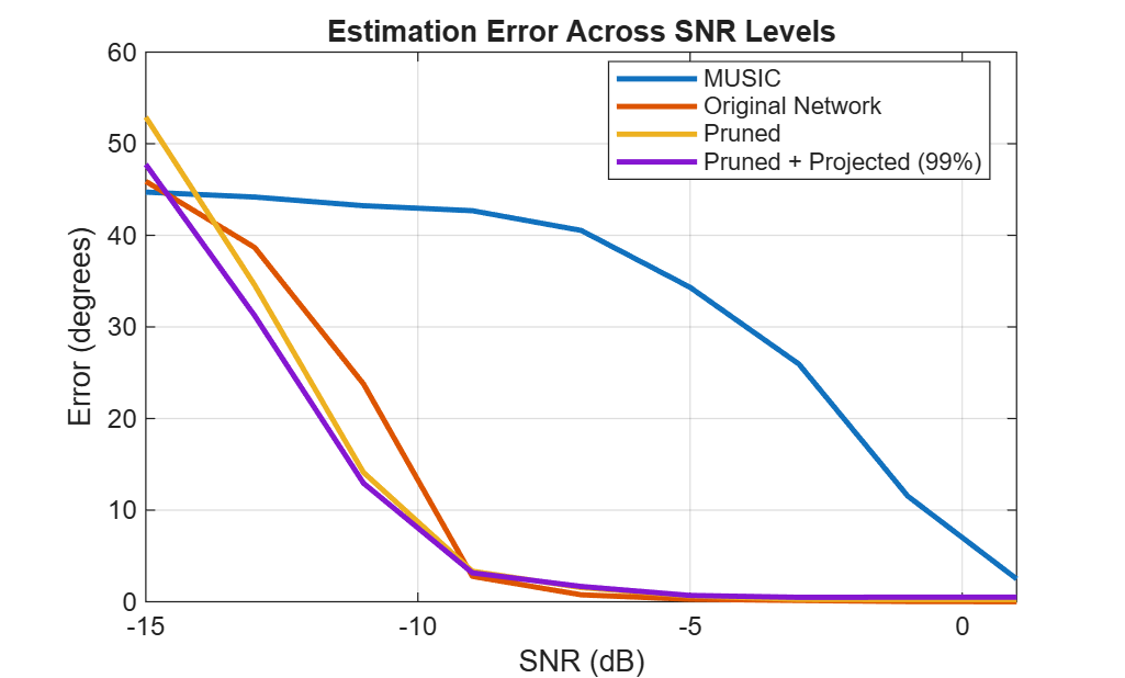
The pruned network maintains comparable accuracy to the original across all SNR levels. At higher variance goals (99%), the projected network closely tracks the pruned network. You can experiment with lower variance goals (such as 0.95) for greater compression, though this introduces accuracy degradation at low SNRs.
Compare Inference Time
Measure the average inference time per sample for the original and compressed networks to quantify the speedup achieved through compression.
testSample = dataset.trainData(:,:,:,10);

tOriginal = timeit(@() predict(deepDOAEstimator, testSample));
tCompressed = timeit(@() predict(prunedAndProjectedNet, testSample));

inferenceTable = table( ...
    [tOriginal*1000; tCompressed*1000], ...
    [1; tOriginal/tCompressed], ...
    VariableNames=["Inference time (ms)", "Speedup"], ...
    RowNames=["Original", "Compressed"]);
disp(inferenceTable)
                  Inference time (ms)    Speedup
                  ___________________    _______

    Original            4.0468                1
    Compressed           2.131            1.899
The compressed network achieves a measurable speedup over the original, as shown in the table above.
Visual Comparison: Compressed Network vs. MUSIC
Randomly select observations from the validation set and compare the MUSIC pseudospectrum with the compressed DOA estimator probability vector. The dotted lines mark the true angle locations.
rng("default");
idxToCompare = randi(length(dataset.validIdx), [1,4]);
helperPlotDOASpectrum(prunedAndProjectedNet, dataset, idxToCompare)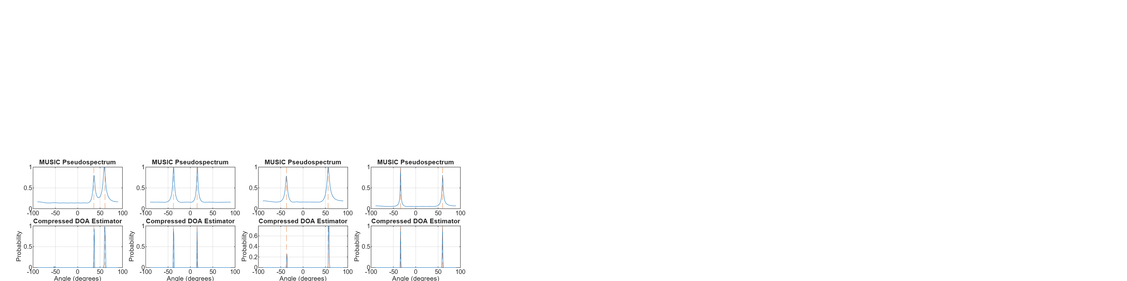
The compressed network produces sharp peaks at the true source locations, demonstrating that pruning and projection preserve the estimation capability of the original network.
The compressed network is compatible with code generation and can be used directly in the Deploy Direction of Arrival Estimation Using Deep Learning on Desktop and Deploy Direction of Arrival Estimation Using Deep Learning on Raspberry Pi examples for efficient real-time deployment.
Helper Functions
function loss = customLoss(y,t)
    loss = crossentropy(y,t,t*10+1,ClassificationMode="multilabel");
end
modelLossPruning computes the loss and gradients required for Taylor-score-based pruning.
function [loss,pruningActivations,pruningGradients,netGradients,state] = modelLossPruning(prunableNet, X, T)
    [dlYPred,state,pruningActivations] = forward(prunableNet,X);
    loss = customLoss(dlYPred,T);
    [pruningGradients,netGradients] = dlgradient(loss, ...
        pruningActivations, prunableNet.Learnables);
end
helperCompareNetworksDOAOverSNR compares DOA estimation error across SNR levels for multiple networks and the MUSIC algorithm.
function helperCompareNetworksDOAOverSNR(doaNetworks, displayNames, dBSNRList, sourceAngles)
    noisePowerList = db2pow(-dBSNRList);
    nsamples = 500;
    scanAngles = -90:90;
    fc = 300e6;
    lambda = physconst("LightSpeed")/fc;
    ula = phased.ULA(NumElements=8, ElementSpacing=lambda/2);

    nSettings = length(noisePowerList);
    signalTest = cell(nSettings*nsamples, 1);
    scovTest = cell(nSettings*nsamples, 1);
    anglesTest = cell(nSettings*nsamples, 1);
    n = 0;

    for ii = 1:nSettings
        noisePower = noisePowerList(ii);
        for jj = 1:nsamples
            n = n + 1;
            [signal, scov] = helperGenerateTestData( ...
                SourceAngles=sourceAngles, ...
                NoisePower=noisePower, ...
                NumSnapshots=500, ULA=ula);
            signalTest{n} = signal;
            scovTest{n} = cat(3, real(scov), imag(scov));
            anglesTest{n} = sourceAngles;
        end
    end

    musicEstimator = phased.MUSICEstimator(SensorArray=ula, ...
        OperatingFrequency=fc, ...
        ScanAngles=scanAngles, ...
        DOAOutputPort=true, ...
        NumSignalsSource="Property", NumSignals=2);
    detectedAnglesMUSIC = cell(length(anglesTest), 1);
    for ii = 1:length(signalTest)
        [~, ang] = musicEstimator(signalTest{ii});
        detectedAnglesMUSIC{ii} = sort(ang);
    end

    scovTensor = dlarray(cat(4, scovTest{:}), "SSCB");
    detectedAnglesDeep = cell(1, length(doaNetworks));
    for ii = 1:length(doaNetworks)
        probVec = minibatchpredict(doaNetworks{ii}, scovTensor);
        detectedAnglesDeep{ii} = helperEstimateAngles(probVec, scanAngles, NumSignalsSource=2);
    end

    errorMUSIC = cellfun(@(x,y) sum(abs(x-y)), detectedAnglesMUSIC, anglesTest);
    errorMUSIC = mean(reshape(errorMUSIC, nsamples, []), 1);

    figure
    plot(dBSNRList, errorMUSIC, LineWidth=2, DisplayName="MUSIC")
    hold on
    for ii = 1:length(doaNetworks)
        errorDeep = cellfun(@(x,y) sum(abs(x-y)), detectedAnglesDeep{ii}, anglesTest);
        errorDeep = mean(reshape(errorDeep, nsamples, []), 1);
        plot(dBSNRList, errorDeep, LineWidth=2, DisplayName=displayNames(ii))
    end
    hold off
    grid on
    box on
    ylabel("Error (degrees)")
    xlabel("SNR (dB)")
    title("Estimation Error Across SNR Levels")
    legend(Location="best")
    xlim([dBSNRList(1) dBSNRList(end)])
end
helperEstimateAngles estimates signal source arrival angles from the network probability vector output.
function Angles = helperEstimateAngles(probVec, angleRes, nvargs)
    arguments
        probVec
        angleRes (:,1) double {mustBeNonempty, mustBeFinite, mustBeVector}
        nvargs.NumSignalsSource = []
        nvargs.Threshold = 0.5
    end

    if isa(probVec, "dlarray")
        probVec = extractdata(probVec);
    end
    Angles = cell(size(probVec,2), 1);
    for ii = 1:size(probVec,2)
        provec = probVec(:,ii);
        [peaks, locs] = findpeaks(provec, angleRes);

        if isempty(nvargs.NumSignalsSource)
            idx = find(peaks > nvargs.Threshold);
        else
            if numel(peaks) < nvargs.NumSignalsSource
                [~, idx] = maxk(peaks, min(numel(peaks), nvargs.NumSignalsSource));
            else
                [~, idx] = maxk(peaks, nvargs.NumSignalsSource);
            end
        end

        angles = sort(locs(idx));
        Angles{ii} = angles(:)';
    end
end
helperGenerateTrainData generates training data for the deep DOA estimator using Phased Array System Toolbox simulations.
function dataStruct = helperGenerateTrainData()
    fc = 300e6;
    lambda = physconst("LightSpeed")/fc;
    ula = phased.ULA(NumElements=8, ElementSpacing=lambda/2);
    nsnapshots = 200;
    angleGrid = -90:1:90;

    rng("default")
    [dataStruct.signalsTrain, scovsTrain, dataStruct.anglesTrain] = ...
        helperGenerateULAData(NoisePower=[0,1,2,5], ...
        Shuffle=true, ULA=ula, Nsnapshots=nsnapshots);

    ndata = length(dataStruct.anglesTrain);
    dataStruct.sigCov = zeros([size(dataStruct.signalsTrain,2), ...
        size(dataStruct.signalsTrain,2), 2, size(dataStruct.signalsTrain,3)]);
    dataStruct.sigCov(:,:,1,:) = real(scovsTrain);
    dataStruct.sigCov(:,:,2,:) = imag(scovsTrain);

    anglesBinaryVec = zeros([length(angleGrid), size(dataStruct.signalsTrain,3)]);
    for ii = 1:ndata
        angleSet = dataStruct.anglesTrain{ii};
        anglesBinaryVec(:,ii) = ismember(angleGrid, angleSet);
    end

    N = ndata;
    trainIdx = 1:floor(0.8*N);
    dataStruct.validIdx = floor(0.9*N)+1:N;

    dataStruct.trainData = dlarray(dataStruct.sigCov(:,:,:,trainIdx), "SSCB");
    dataStruct.trainLabels = dlarray(anglesBinaryVec(:,trainIdx), "CB");
    dataStruct.validData = dlarray(dataStruct.sigCov(:,:,:,dataStruct.validIdx), "SSCB");
    dataStruct.validLabels = dlarray(anglesBinaryVec(:,dataStruct.validIdx), "CB");
end
helperGenerateULAData generates ULA signal data using Phased Array System Toolbox.
function [Signals, Scovs, Angles] = helperGenerateULAData(nvargs)
    arguments
        nvargs.NoisePower = 1
        nvargs.ULA = []
        nvargs.Fc = 300e6
        nvargs.NAngles = 181
        nvargs.NSources = [1 2]
        nvargs.Shuffle logical = true
        nvargs.Nsnapshots = 200
    end

    fc = nvargs.Fc;
    ula = nvargs.ULA;
    Nelements = ula.NumElements;
    lambda = physconst("LightSpeed")/fc;
    pos = getElementPosition(ula) / lambda;

    noisePwrs = nvargs.NoisePower;
    nangle = nvargs.NAngles;
    angleRes = linspace(-90, 90, nangle);
    angleCombsList = cell(length(nvargs.NSources), 1);
    for ii = 1:length(nvargs.NSources)
        nsources = nvargs.NSources(ii);
        angleCombs = nchoosek(angleRes, nsources);
        angleCombsList{ii} = mat2cell(angleCombs, ones(1,size(angleCombs,1)), nsources);
    end
    angleCombsAll = cat(1, angleCombsList{:});

    if nvargs.Shuffle
        angleCombsAll = angleCombsAll(randperm(size(angleCombsAll, 1)), :);
    end

    Nsnapshots = nvargs.Nsnapshots;
    nsnr = length(noisePwrs);
    Signals = zeros(Nsnapshots, Nelements, size(angleCombsAll,1)*nsnr);
    Scovs = zeros(Nelements, Nelements, size(angleCombsAll,1)*nsnr);
    Angles = cell(size(angleCombsAll,1)*nsnr, 1);

    for ii = 1:size(angleCombsAll, 1)
        az_ang = angleCombsAll{ii,:};
        el_ang = zeros(1, numel(az_ang));
        for jj = 1:nsnr
            noisePwr = noisePwrs(jj);
            [signal,~,scov] = sensorsig(pos, Nsnapshots, [az_ang; el_ang], noisePwr);
            idx = (ii-1)*nsnr + jj;
            Signals(:,:,idx) = signal;
            Scovs(:,:,idx) = scov;
            Angles{idx} = az_ang;
        end
    end
end
helperGenerateTestData generates test data for DOA estimation evaluation.
function [Signals, Scovs] = helperGenerateTestData(nvargs)
    arguments
        nvargs.NumElements = 8
        nvargs.NumSnapshots = 100
        nvargs.NoisePower = 1
        nvargs.ULA = []
        nvargs.Fc = 300e6
        nvargs.SourceAngles = []
    end

    fc = nvargs.Fc;
    lambda = physconst("LightSpeed")/fc;

    if isempty(nvargs.ULA)
        ula = phased.ULA(NumElements=nvargs.NumElements, ElementSpacing=lambda/2);
    else
        ula = nvargs.ULA;
    end
    pos = getElementPosition(ula) / lambda;

    az_ang = nvargs.SourceAngles;
    el_ang = zeros(1, length(az_ang));
    [Signals,~,Scovs] = sensorsig(pos, nvargs.NumSnapshots, ...
        [az_ang; el_ang], nvargs.NoisePower);
end
helperPlotDOASpectrum plots the MUSIC pseudospectrum and deep DOA estimator probability vector for visual comparison.
function helperPlotDOASpectrum(deepDOAEstimator, dataStruct, idxList)
    fc = 300e6;
    lambda = physconst("LightSpeed")/fc;
    ula = phased.ULA(NumElements=8, ElementSpacing=lambda/2);
    scanAngles = linspace(-90, 90, 181);

    musicEstimator = phased.MUSICEstimator(SensorArray=ula, ...
        OperatingFrequency=fc, ...
        ScanAngles=scanAngles, ...
        DOAOutputPort=true, ...
        NumSignalsSource="Property", NumSignals=2);

    figure(Position=[0 0 2000 500])
    tiledlayout(2, length(idxList))
    colors = lines(2);
    for ii = 1:length(idxList)
        idx = dataStruct.validIdx(idxList(ii));
        signal = dataStruct.signalsTrain(:,:,idx);
        [ymusic,~] = musicEstimator(signal);
        scov = dataStruct.sigCov(:,:,:,idx);
        probVec = minibatchpredict(deepDOAEstimator, dlarray(scov,"SSCB"));

        nexttile(ii)
        plot(scanAngles, ymusic./max(ymusic))
        title("MUSIC Pseudospectrum")
        xline(dataStruct.anglesTrain{idx}, "--", Color=colors(2,:))
        grid on
        box on

        nexttile(ii + length(idxList))
        plot(scanAngles, probVec)
        xline(dataStruct.anglesTrain{idx}, "--", Color=colors(2,:))
        title("Compressed DOA Estimator")
        xlabel("Angle (degrees)")
        ylabel("Probability")
        box on
        grid on
    end
end
See Also
Topics
- Direction-of-Arrival Estimation Using Deep Learning
- Build and Deploy Your First Simulink Model to Raspberry Pi (Raspberry Pi Blockset)
- Deploy Direction of Arrival Estimation Using Deep Learning on Desktop
- Deploy Direction of Arrival Estimation Using Deep Learning on Raspberry Pi
- Deploy Direction of Arrival Estimation Using a PyTorch Model on Raspberry Pi

