System Identification Using LMS Filter Block
R2026bThis example shows how to identify an unknown FIR system using the LMS Filter block in DSP HDL Toolbox™. A unit-power random signal drives both an unknown 16-tap FIR filter and a LMS Filter block configured for the transposed form delayed least mean square (LMS) architecture. As the adaptive filter converges, its estimated coefficients match the actual system coefficients, demonstrating hardware-efficient system identification. In this example, you configure a transposed form delayed LMS filter for hardware-efficient system identification, observe convergence of the adaptive filter by comparing estimated and actual coefficients, and verify the Simulink® block outputs against the dsp.LMSFilter reference function.
Configure Unknown System and Input Signals
To perform system identification, you need a reference system whose coefficients the adaptive filter attempts to learn. The unknown system is a 16-tap FIR lowpass filter designed with fircband. The filter length of 16 balances sufficient spectral shaping with manageable hardware resource usage in the adaptive filter.
filterLength = 16;
filterObj = dsp.FIRFilter;
filterObj.Numerator = fircband(filterLength-1, [0 0.4 0.5 1], ...
    [1 1 0 0], [1 0.2], {"w", "c"});
The input signal is a unit-power Gaussian random sequence of 1500 samples. A random signal excites all frequency bands equally, which ensures the adaptive filter can identify the full frequency response of the unknown system. The desired signal is the output of the unknown FIR filter plus a small amount of additive noise.
observedSignal = randn(1500, 1);
noise = 0.01*randn(1500, 1);
desiredSignal = filterObj(observedSignal) + noise;
Set Step Size and Control Signals
The step size controls the tradeoff between convergence speed and steady-state error. A step size of 0.01 provides stable convergence for a 16-tap filter driven by a unit-power signal. Larger values converge faster but produce higher residual error, while smaller values converge more slowly but track the unknown system more precisely.
stepSize = 0.01;
The control signals determine when the filter adapts and processes valid data. Setting adaptIn to true means the filter updates its weights on every sample. Setting validIn to true indicates every input sample is valid. Setting resetIn to false means the filter never resets during operation.
adaptIn = true(length(observedSignal), 1);
resetIn = false(length(observedSignal), 1);
validIn = true(length(observedSignal), 1);
Calculate Simulation Time and Run Model
The transposed form delayed LMS architecture introduces pipeline latency to achieve higher clock rates in hardware. You must account for this latency when setting the simulation stop time to ensure all input samples produce corresponding outputs. The getLatency method returns the exact pipeline delay for your filter configuration.
lmsObj = dsphdl.LMSFilter(Architecture="Transposed form delayed LMS", ...
    FilterLength=filterLength);
lmsLatency = getLatency(lmsObj);
simtime = length(observedSignal) + lmsLatency + 10;
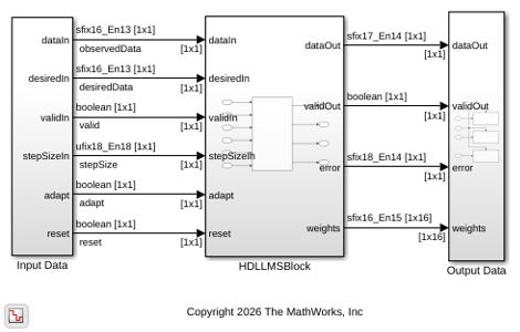
Run the simulation. The model reads  ,
,  ,
,  , and the control signals from the base workspace.
modelname = "HDLTransposedDelayedLMS";
open_system(modelname);
out = sim(modelname);
Extract the valid output data. The squeeze function removes singleton dimensions from the logged signals.
actFilterOut = squeeze(out.filterOut);
actCoeffOut = squeeze(out.coeffOut)';
actErrorOut = squeeze(out.errorOut);
actFilterOut = actFilterOut(1:length(observedSignal));
actErrorOut = actErrorOut(1:length(observedSignal));
actCoeffOut = actCoeffOut(1:length(observedSignal), :);
Observe Filter Convergence
To verify that the adaptive filter converges, plot the desired signal, filter output, and error signal over time. As the LMS algorithm adapts, the filter output tracks the desired signal and the error signal decreases toward zero.
figure;
plot(1:length(observedSignal), ...
    double([desiredSignal, actFilterOut, actErrorOut]))
title("System Identification of FIR Filter")
legend("Desired", "Output", "Error")
xlabel("Time Index")
ylabel("Signal Value")
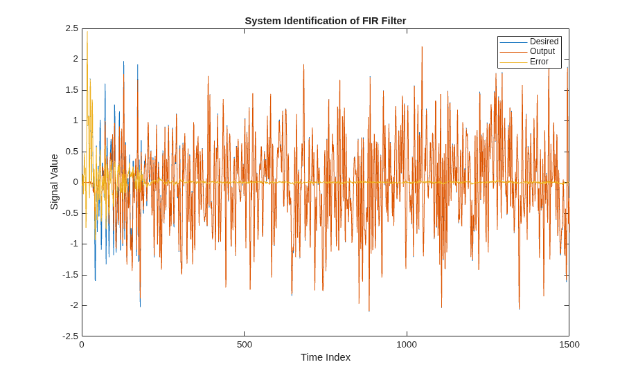
The error signal starts large when the filter weights are initialized to zero. Over time, the error decreases as the adaptive filter learns the unknown system coefficients. The filter output increasingly overlaps with the desired signal, confirming convergence. To confirm that the adaptive filter has identified the unknown system, compare the actual FIR filter coefficients with the estimated weights at the end of the simulation. If the system identification succeeds, the two sets of coefficients match closely.
finalIdx = length(observedSignal);
figure;
stem([(filterObj.Numerator).', double(actCoeffOut(finalIdx, :)).'])
xlabel("Coefficient Index")
ylabel("Coefficient Value")
title("Actual vs. Estimated Filter Weights")
legend("Actual","Estimated", 'Location', 'northeast');
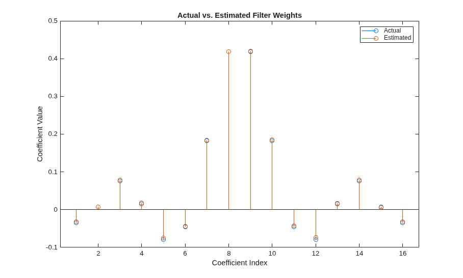
The stem plot shows the estimated weights closely matching the actual FIR filter coefficients. Small residual differences result from the additive noise and the finite convergence time. Increasing the number of input samples or decreasing the step size reduces these differences at the cost of longer adaptation time.
Verify Against Reference LMS Function
To confirm that the HDL-optimized block produces correct results, compare its outputs against the dsp.LMSFilter reference function. The reference function implements the same algorithm without hardware pipeline delays, so matching outputs validate the block's numerical behavior.
lmsRef = dsp.LMSFilter(filterLength, StepSize=stepSize);
[refFilterOut, refErrorOut, refCoeffOut] = ...
    lmsRef(observedSignal, desiredSignal);

figure;
subplot(3, 1, 1)
plot(1:length(observedSignal), [actFilterOut, refFilterOut])
title("Comparison Between Simulink and Reference Outputs")
subtitle("Filter Output")
legend("Simulink filter output", "Reference filter output", ...
    Location="bestoutside")
xlabel("Time Index")
ylabel("Signal Value")

subplot(3, 1, 2)
plot(1:length(observedSignal), [actErrorOut, refErrorOut])
subtitle("Error Output")
legend("Simulink error output", "Reference error output", ...
    Location="bestoutside")
xlabel("Time Index")
ylabel("Signal Value")

subplot(3, 1, 3)
plot(1:filterLength, ...
    [double(actCoeffOut(finalIdx, :)).', refCoeffOut])
subtitle("Coefficients Output")
legend("Simulink coefficients", "Reference coefficients", ...
    Location="bestoutside")
xlabel("Coefficient Index")
ylabel("Coefficient Value")
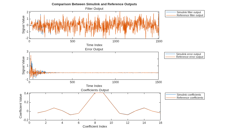
The Simulink block outputs match the reference function outputs. The filter output and error signals overlap across all 1500 time steps, and the final estimated coefficients align closely. This confirms that the transposed form delayed LMS architecture in the LMS Filter block produces numerically equivalent results to the floating-point reference, while offering an architecture suitable for HDL code generation.

