C Code Optimization using Codegen for Qualcomm Hexagon DSP
This example demonstrates the workflow of generating optimized C code in MATLAB® using Codegen for the Qualcomm Hexagon Simulator.
The example utilizes a dsp.FIRFilter System object to filter two sine waves with different frequencies using the Embedded Coder® Support Package for Qualcomm® Hexagon® Processors and the Qualcomm Hexagon QHL Code Replacement Library (CRL).
Supported Hardware
Qualcomm Hexagon Simulator
Qualcomm Hexagon Android Board
Prerequisites
Launch the hardware setup and install the Qualcomm SDK. For more information, see Launch Hardware Setup.
Required Hardware
To run this example, you need the following hardware:
Qualcomm Hexagon Simulator
Create MATLAB Coder Configuration Object
Create MATLAB Coder configuration object by running this code on MATLAB command.
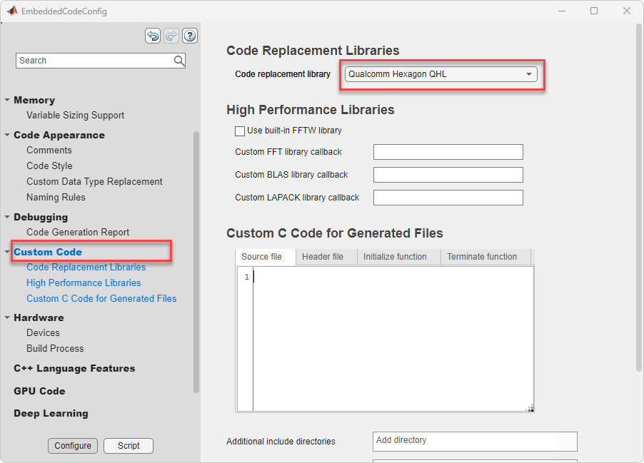
cfg = coder.config('lib','ecoder',true);

% Configure the hardware and select the processor_version
cfg.Hardware = coder.Hardware('Qualcomm Hexagon Simulator');
cfg.Hardware.CPUClockRate = 300;
cfg.Hardware.ProcessorVersion = 'V68';
cfg.CodeReplacementLibrary = "Qualcomm Hexagon QHL";
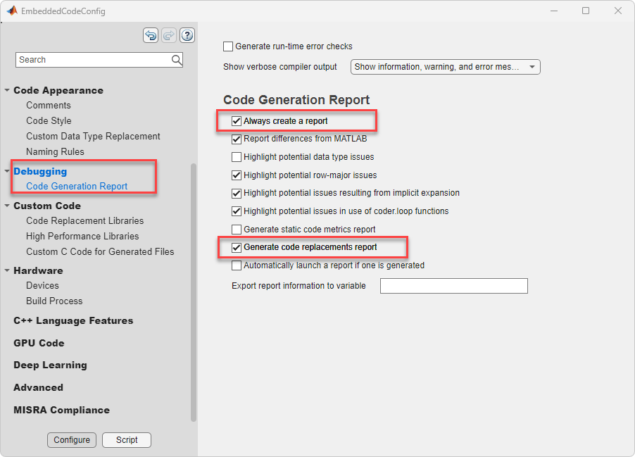
Enable code replacement report, useful to analyze the replacement functions
cfg.GenerateCodeReplacementReport = true;
Optionally for PIL verification, set the these configuration
cfg.VerificationMode = "PIL";
cfg.CodeExecutionProfiling = true;
To generate report with Hexagon Profiler or gprof, set the cfg.Hardware.Profiler to one of the following.
None
Hexagon Profiler
gprof
Hexagon Profiler and gprof
Optionally, simulator options can be provided using cfg.Hardware.SimulatorOptions. For more information, refer to the Hexagon Simulator documentation. Similarly, hexagon profiler options can be provided using cfg.Hardware.ProfilerOptions. For more information, refer to the Hexagon Profiler documentation.
Alternatively, the configuration object can also be configured using the GUI with the cfg.dialog command. The settings can then be configured in the same way as the steps mentioned in the 'Generate C Code' section of the C Code Optimization Using MATLAB Coder App for Hexagon DSP example.
Generate Code
Run this command to generate code and launch the code generation report.
numSamples = 160;
codegen -config cfg ex_fir_hexagon_ml -args {zeros(numSamples,1,'single')} -launchreport
### Printing set environment variables:
### Connectivity configuration for function 'ex_fir_hexagon_ml': 'Hexagon Simulator'
Code generation successful: View report

To view the replacement hits, navigate to the summary section and click on Code Replacements.

Numerical verification
To verify numerical accuracy, you need a test script that compares the MATLAB implementation output with the output of the generated PIL MEX file.
sin1 = dsp.SineWave('Amplitude',1,'Frequency',1000,...
                     'SampleRate',16000, 'SamplesPerFrame', numSamples,...
                     'OutputDataType', 'single');
sin2 = dsp.SineWave('Amplitude',4,'Frequency',5000,...
                     'SampleRate',16000, 'SamplesPerFrame', numSamples,...
                     'OutputDataType', 'single');

numSteps = 200;
frameLength = sin1.SamplesPerFrame;
yRef = zeros(frameLength,1,numSteps,'single');
y = zeros(frameLength,1,numSteps,'single');

for k = 1:numSteps
   x1k = sin1(); % generate 1KHz sine wave
   x5k = sin2(); % generate 5KHz sine wave
   n = randn(size(x1k), 'single')*sqrt(.05); % generate noise signal
   u = x1k+x5k+n;
   % Run with MATLAB code on host machine
   yRef(:,:,k) = ex_fir_hexagon_ml(u);
   % Run with generated code on target
   y(:,:,k) = ex_fir_hexagon_ml_pil(u);
end
### Starting application: 'codegen\lib\ex_fir_hexagon_ml\pil\ex_fir_hexagon_ml'
    To terminate execution: clear ex_fir_hexagon_ml_pil
    Execution profiling data is available for viewing. Open Simulation Data Inspector.
    Execution profiling report will be available after termination.
clear ex_fir_hexagon_ml;
clear ex_fir_hexagon_ml_pil;
### Stopping application.
Output logs
Error logs
    Execution profiling report: coder.profile.show(getCoderExecutionProfile('ex_fir_hexagon_ml'))
After execution, you can compare the outputs of the PIL against the reference using any norm function.
% norm comparison of y & yRef
absoluteError = norm(y(:)-yRef(:),'inf');
fprintf("Absolute error = %g \n",absoluteError);
Absolute error = 9.53674e-07
Alternatively, you can use the verifyEqual function from the matlab.unittest.TestCase.forInteractiveUse test class. This function allows you to compare the outputs against the given absolute and relative tolerances, concluding the overall results.
reltol = single(1e-5);
abstol = single(1e-5);
matlab.unittest.TestCase.forInteractiveUse.verifyEqual(y,yRef, ...
    'RelTol',reltol, 'AbsTol', abstol);
Verification passed.
Similar to Simulink PIL, you can use the Simulation Data Inspector to visualize and compare the previously mentioned outputs. To achieve this, represent the output in the timeseries format.
% Create a timeseries
timeSteps = 1:numSteps;
yTS = timeseries(y,timeSteps,"Name","PIL output(y)");
yRefTS = timeseries(yRef,timeSteps,"Name","MATLAB output (yRef)");

% open Simulation data inspector
Simulink.sdi.view
To import the earlier time series data into the Simulation Data Inspector, select Import. In the Import dialog box, you can choose to import data from the workspace.
After importing, set the yRef to Set as Baseline and y to Set as Compare to.
After importing and configuring the baseline and compare-to settings, navigate to the Compare tab in the SDI. To set the tolerance limit, set Global Tolerances under the Options dropdown. Click Compare to visualize the output of each sample at each time step.

Analyze Performance using Code Profile Analyzer
Run this command to show the coder execution profile.
coder.profile.show(getCoderExecutionProfile('ex_fir_hexagon_ml'))
Consider the average execution time of the ex_fir_hexagon_ml function which is 57,549 cycles. Now, by repeating the code profiling by changing the Code replacement library to None, the previous function takes 131,980 cycles. This indicates that by enabling the CRL, the cycle performance of the ex_fir_hexagon_ml improved by approximately 2.3 times.
Note: For Qualcomm Hexagon QHL CRL, explicit alignment specification for buffers is necessary only when the input/output variables are directly used in the operators, functions and system-objects.