Create Predictive Vector Autoregression Model Using Econometric Modeler

This example models the quarterly US GDP growth rate, M1 money supply rate, and the 3-month T-bill rate series by using the Econometric Modeler app. The example shows how to perform the following actions in the app:

1. Stabilize the raw nonstationary series.

2. Fit several competing vector autoregression (VAR) models, and choose the one with the best, parsimonious fit.

3. Diagnose each residual series.

4. Export the chosen model to the command line to conduct a Granger-Causality test.

5. Generate MMSE forecasts from the best fitting model using the app.

At the command line, the example conducts Granger-causality tests on the series given the estimated model, and it uses the model to generate forecasts.

The data set, which is stored in Data_USEconModel.mat, contains the raw, quarterly US GDP, M1 money supply, and 3-month T-bill rate, among other series, from 1947 through 2009.

Load and Import Data into Econometric Modeler

At the command line, load the Data_USEconModel.mat data set.

load Data_USEconModel

At the command line, open the Econometric Modeler app.

econometricModeler

Alternatively, open the app from the apps gallery (see Econometric Modeler).

Import DataTimeTable into the app:

1. On the Modeler tab, in the Import section, click the Import button .

2. In the Import Data dialog box, select the check box for the DataTimeTable variable.

3. Click Import.

GDP, M1SL, and TB3MS, among other series, appear in the Time Series pane, and a time series plot containing all series appears in the figure window.

Create separate time series plots by double-clicking each of GDP, M1SL, and TB3MS in the Time Series pane. Position the Plot(series) tabs by clicking and dragging each to see all plots simultaneously.

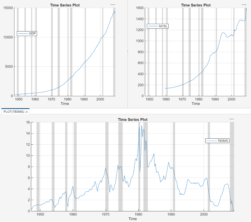
The US GDP and M1 money supply series exhibit exponential growth, and the 3-month T-Bill series appears like a random walk.

Diagnose and Transform Series

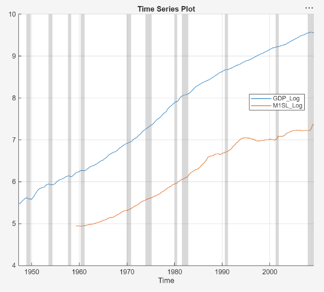
Remove the exponential trend from the GDP and M1 money supply series by applying the log transform to each series. Click the Modeler tab, and then, in the Time Series pane, click GDP and Ctrl click M1SL. In the Transforms section, click Log. The transformed series GDP_Log and M1SL_Log appear in the Time Series pane, and their time series plot appears in the Plot(GDP_Log) figure window.

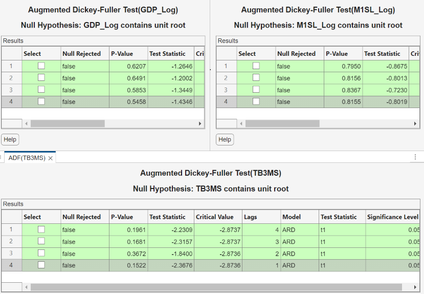
Test the null hypothesis that each series is a unit root process against a stationary AR(p) with drift alternative, where p = 4 through 1. For each series GDP_Log, M1SL_Log, and TB3MS:

1. On the Modeler tab, in the Time Series pane, click the series.

2. On the Modeler tab, in the Time Series pane, click Add Test > Augmented Dickey-Fuller Test.

3. On the ADF tab, in the Settings section, in the Number of Lags box, type 4. In the Model menu, choose Autoregressive with Drift.

4. In the Tests section, click Run.

5. Repeat steps 3 and 4 for lags 3, 2, and 1.

The following figures show the results. The tests fail to reject the null hypotheses of a unit root series in all cases, which suggests that each series is difference stationary.

Stabilize the series by applying the first difference to each series.

1. Click the Modeler tab, and then, in the Time Series pane, click GDP_Log and Ctrl+click M1SL_Log and TB3MS.

2. In the Transforms section, click Difference. The transformed series GDP_Log_Diff, M1SL_Log_Diff, and TB3MS_Diff appear in the Time Series pane, and their time series plot appears in the Plot(GDP_Log_Diff) figure window.

3. Rename GDP_Log_Diff and M1SL_Log_Diff to GDPRate and M1SLRate by clicking their names twice in the Time Series pane, and typing their new names.

Estimate VAR Models

Estimate 3-D VAR(p) models of the US quarterly GDP growth rate series GDPRate, M1 money supply growth rate series M1SLRate, and change in the 3-month treasury bill rate series TB3MS_Diff, where p = 1 through 4.

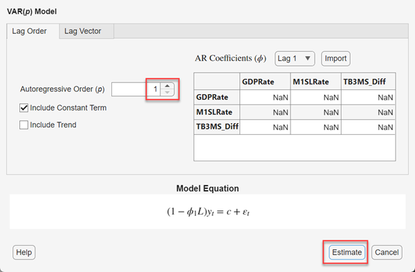
1. In the Time Series pane, click GDPRate and Ctrl+click M1SLRate and TB3MS_Diff.

2. In the Models section, click VAR.

3. Fit a VAR(1) model (the default) by clicking Estimate in the VAR Model Parameters dialog box.

   

   The model variable VAR appears in the Models pane, its value appears in the Preview pane, and its estimation summary appears in the Fit(VAR) document. Change the name of the model variable VAR to VAR_1 by clicking VAR twice in the Models pane, and then typing VAR_1.

4. Repeat steps 1 through 3 for each AR order p = 2 through 4. In the Var Model Parameters dialog box, set the AR order by using the Autoregressive Order (p) box.

   Similar to the VAR(1) estimation, a variable for each model (VAR_2, VAR_3, and VAR_4) appears in the Models pane, and their estimation summaries appear in their respective Fit(ModelName) document. You can view properties of an estimated model in the Preview pane by clicking the model in the Models pane. For example, click VAR_4.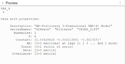

   

Select Model with Best In-Sample Fit

The estimation summary in each Fit(VAR_p) tab contains a plot of fitted values and residuals, with respect to the time series in the Time Series list, a standard statistical table of estimates and inferences, and a table of information criteria.

Compare the information criteria of each estimated model simultaneously by positioning the estimation summary documents so that they occupy the four quadrants of the right pane. The model with the lowest value has the best, parsimonious fit.

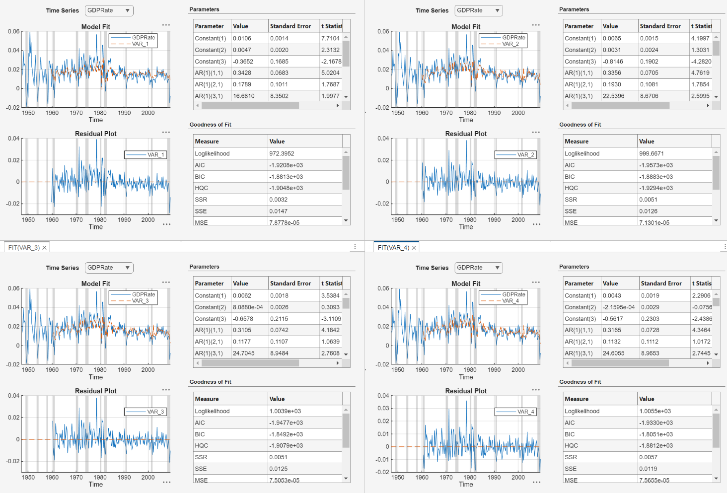
The VAR(2) model VAR_2 produces the lowest AIC and BIC values. Choose this model for further analysis.

Check Goodness of Fit

Inspect the following VAR(2) plots of each residual series:

• Histograms, for center, normality, and outliers

• Quantile-quantile plots, for normality, skewness, and tails

• Autocorrelation function (ACF), for serial correlation

• ACF of squared residual series, for heteroscedasticity

This example diagnoses the residuals visually. Alternatively, you can conduct statistical tests to diagnose the residuals.

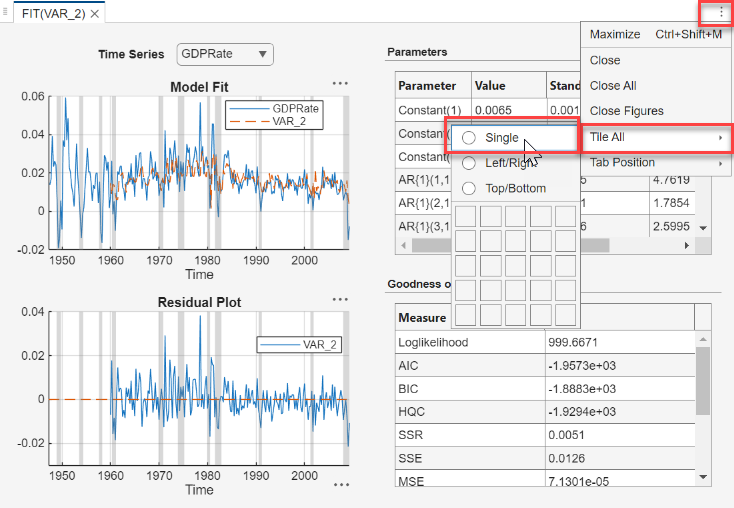
In the Fit(VAR_2) document, click Document Actions > Tile All, and then click the Single radio button.

On the Models pane, click VAR_2.

Plot separate residual histograms. On the Modeler tab, in the Diagnostics section, click Model Fit Diagnostics > Residual Histogram. Histograms of the each residual series appear in the Hist(VAR_2) document.

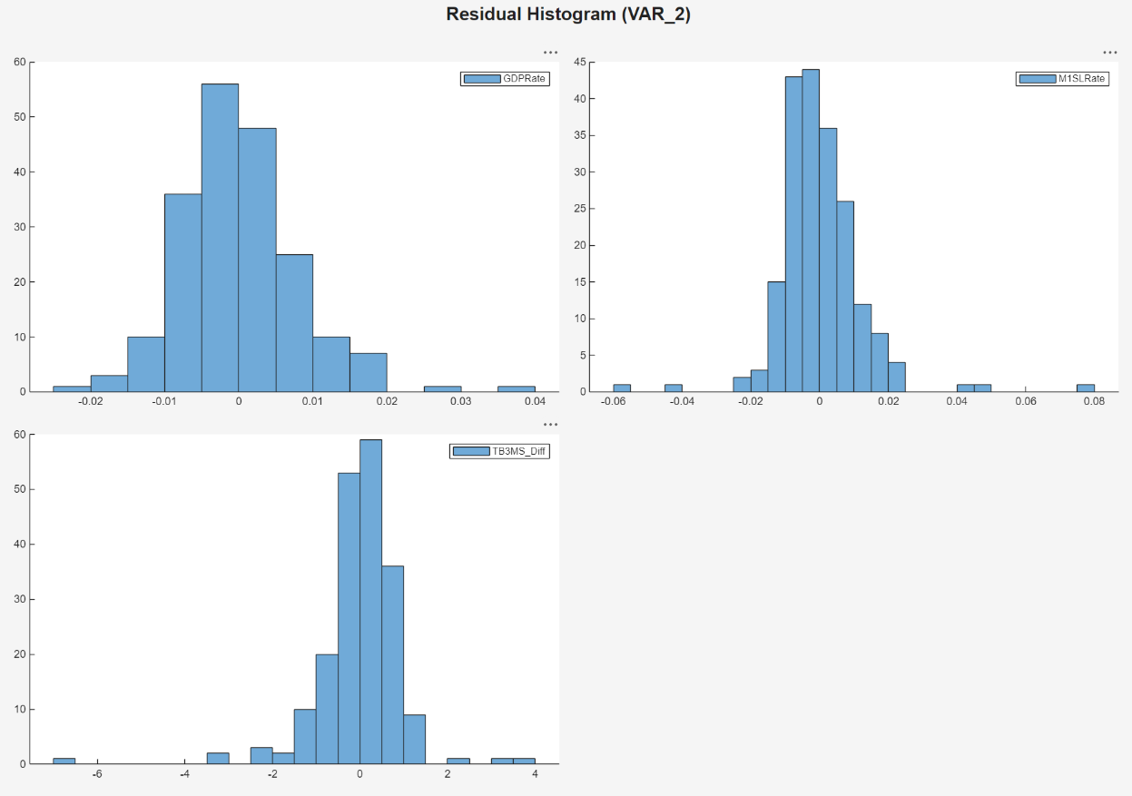
Each residual series appears centered around 0, with varying degrees of slight skewness and possible outliers. This example proceeds without addressing possible skewness and outliers.

Plot separate residual quantile-quantile plots. With VAR_2 selected in the Time Series pane, on the Modeler tab, in the Diagnostics section, click Model Fit Diagnostics > Residual Q-Q Plot. Quantile-quantile plots of each residual series appear in the QQ(VAR_2) document.

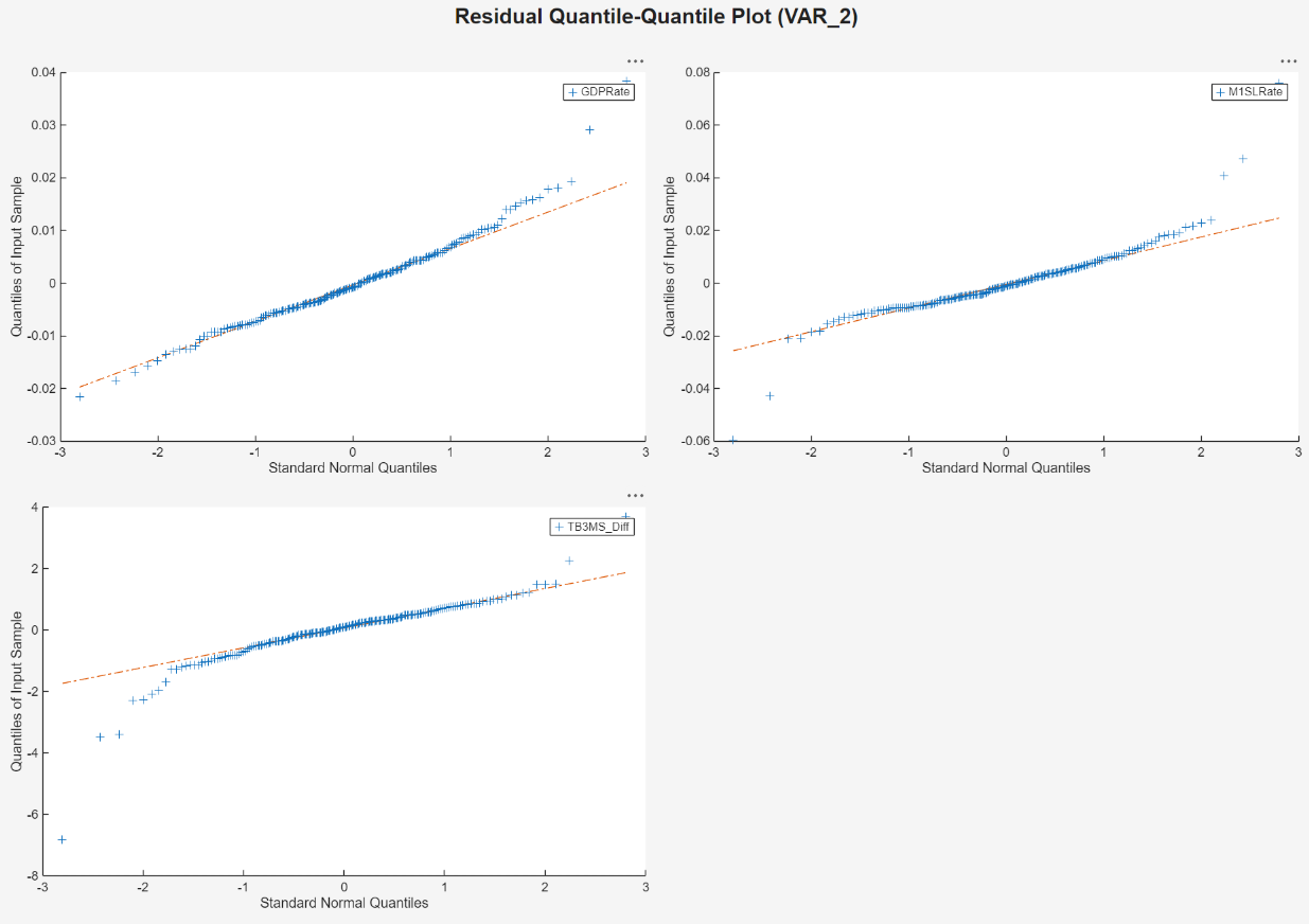
Each series has slightly fatter tails than what is expected by the normal distribution. This example proceeds without addressing possible kurtosis.

Plot separate ACF plots of each residual series. With VAR_2 selected in the Time Series pane, on the Modeler tab, in the Diagnostics section, click Model Fit Diagnostics > Residual Autocorrelation. ACF plots of each residual series appear in the ACF(VAR_2) document.

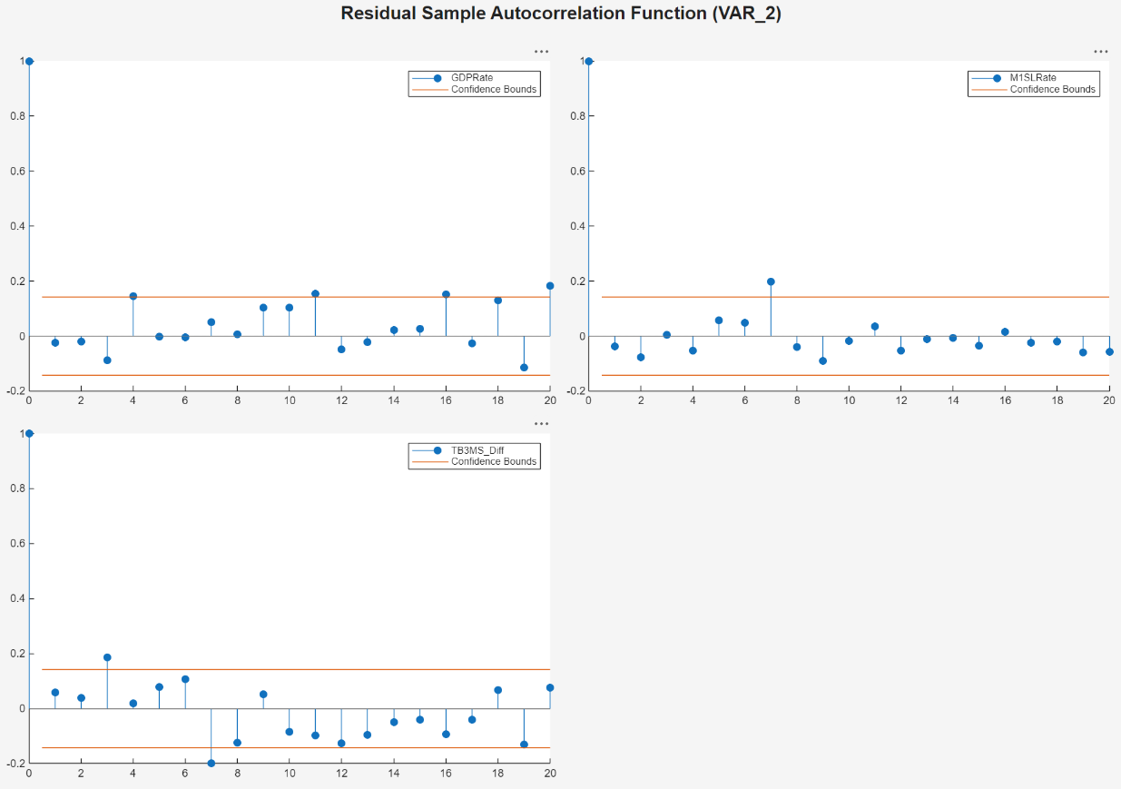
Each series has several significant, albeit small, autocorrelations. For example, the GDPRate residual series has significant autocorrelations at lags 4 and 16, and the M1SLRate and TB3MS_Diff quarterly difference series both have significant autocorrelations at lags 7. To address the autocorrelations, you can include higher AR lags in the VAR model for estimation, but this example proceeds without addressing the autocorrelations this way.

Plot separate ACF plots of each squared residual series. With VAR_2 selected in the Time Series pane, on the Modeler tab, in the Diagnostics section, click Model Fit Diagnostics > Squared Residual Autocorrelation. ACF plots of the each squared residual series appear in the ACF(VAR_2)_2 document.

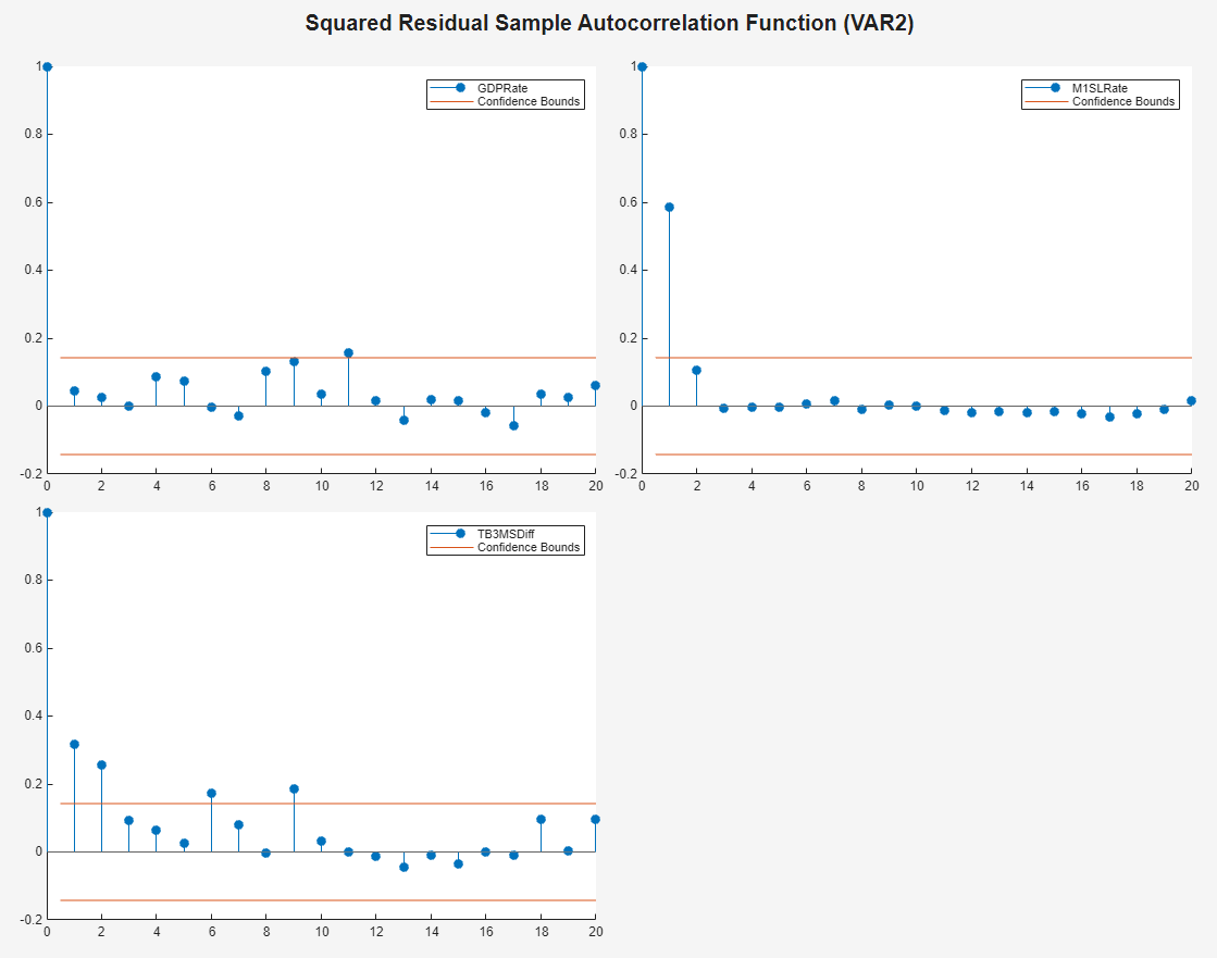
The M1SLRate and TB3MS_Diff series have significant autocorrelations, which suggests that heteroscedasticity is present. This example proceeds without addressing possible heteroscedasticity.

Export Model to Workspace

Export the model to the workspace.

1. With the VAR_2 model selected in the Models pane, on the Modeler tab, in the Export section, click Export > Export Variables.

2. In the Export Variables dialog box, select the Select check box for GDPRate, M1SLRate, and TB3MS_Diff.

3. Click Export.

The variables GDPRate, M1SLRate, TB3MS_Diff, and VAR_2 appear in the workspace.

Conduct Causality Analysis at Command Line

Determine whether series in the system Granger-cause the other series by conducting 1-step, leave-one-out Granger-causality tests. Pass the estimated VAR(2) model to gctest.

gctest(VAR_2)

                          H0                                Decision         Distribution    Statistic      PValue      CriticalValue
    _______________________________________________    __________________    ____________    _________    __________    _____________

    "Exclude lagged M1SLRate in GDPRate equation"      "Reject H0"            "Chi2(2)"        8.3934       0.015045       5.9915    
    "Exclude lagged TB3MSDiff in GDPRate equation"     "Reject H0"            "Chi2(2)"        16.924     0.00021133       5.9915    
    "Exclude lagged GDPRate in M1SLRate equation"      "Cannot reject H0"     "Chi2(2)"        3.1528        0.20672       5.9915    
    "Exclude lagged TB3MSDiff in M1SLRate equation"    "Reject H0"            "Chi2(2)"        20.855     2.9608e-05       5.9915    
    "Exclude lagged GDPRate in TB3MSDiff equation"     "Reject H0"            "Chi2(2)"        20.565     3.4229e-05       5.9915    
    "Exclude lagged M1SLRate in TB3MSDiff equation"    "Cannot reject H0"     "Chi2(2)"       0.41428        0.81291       5.9915    

The null hypothesis of the 1-step leave-one-out Granger-causality test is that a series does not 1-step Granger-cause another series, conditioned on all other series being present in the system. The results suggest:

• Given that the 3-month T-bill change is in the system, enough evidence exists to suggest that M1 money supply rate 1-step Granger-causes the GDP rate.

• Given that the M1 money supply rate is in the system, enough evidence exists to suggest that the 3-month T-bill change 1-step Granger-causes the GDP rate.

• Given that the 3-month T-bill change is in the system, not enough evidence exists to suggest that the GDP rate 1-step Granger-causes the M1 money supply rate.

• Given that the GDP rate is in the system, enough evidence exists to suggest that the 3-month T-bill change 1-step Granger-causes the M1 money supply rate.

• Given that the M1 money supply rate is in the system, enough evidence exists to suggest that the GDP rate 1-step Granger-causes the 3-month T-bill change.

• Given that the GDP rate is in the system, not enough evidence exists to suggest that the 1-step M1 money supply rate Granger-causes the 3-month T-bill change.

Generate Forecasts Using Econometric Modeler

Generate MMSE forecasts and approximate 95% forecast intervals from the estimated VAR(2) model for the next four years (16 quarters).

1. From the Econometric Modeler app, in the Models pane, select the VAR_2 model.

2. In the Modeler tab, in the Forecast section, click Forecast.

3. In the Forecast Model Response dialog box, set Number of periods in forecast horizon to 16. Then, click Forecast.

   

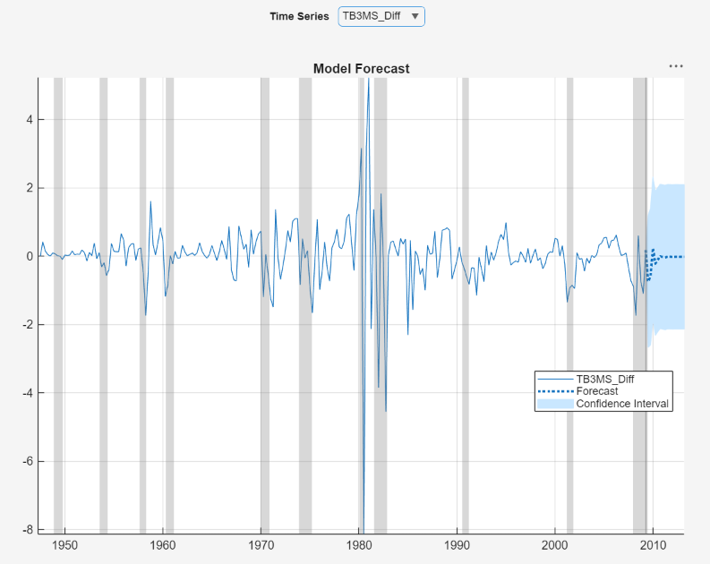
In the right pane, in the For(VAR_2) tab is a figure window of a plot of the GDPRate series with forecasts and 95% forecast intervals at the end of the series, generated from the VAR(2) model.

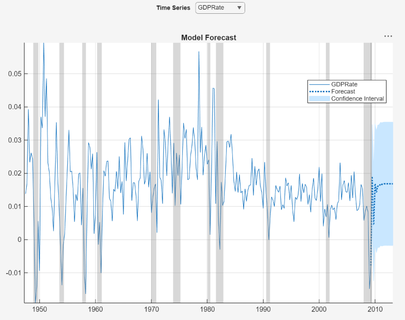
To display the forecasts of the other variables in the VAR(2) model, use the Time Series menu in the figure window. For example, display the forecasts of the TB3MS_Diff series, in the figure window, click Time Series > TB3MS_Diff.