summarize
Summarize threshold-switching dynamic regression model estimation results
Since R2021b
Description
summarize( displays a summary of the
threshold-switching dynamic regression model Mdl)Mdl.
If
Mdlis an estimated model returned byestimate, thensummarizedisplays estimation results to the MATLAB® Command Window. The display includes:A model description
Estimated threshold transitions
Fit statistics, which include the effective sample size, number of estimated submodel parameters and constraints, loglikelihood, and information criteria (AIC and BIC)
A table of submodel estimates and inferences, which includes coefficient estimates with standard errors, t-statistics, and p-values
If
Mdlis an unestimated threshold-switching model returned bytsVAR,summarizeprints the standard object display (the same display thattsVARprints during model creation).
results = summarize(___)
If
Mdlis an estimated threshold-switching model,resultsis a table containing the submodel estimates and inferences.If
Mdlis an unestimated model,resultsis atsVARobject that is equal toMdl.
summarize does not print to the Command Window
Examples
Assess estimation accuracy using simulated data from a known data-generating process (DGP). This example uses arbitrary parameter values.
Create Model for DGP
Create a discrete threshold transition at mid-level 1.
ttDGP = threshold(1)
ttDGP =
  threshold with properties:

          Type: 'discrete'
        Levels: 1
         Rates: []
    StateNames: ["1"    "2"]
     NumStates: 2
ttDGP is a threshold object representing the state-switching mechanism of the DGP.
Create the following fully specified self-exciting TAR (SETAR) model for the DGP.
State 1: .
State 2: .
.
Specify the submodels by using arima.
mdl1DGP = arima(Constant=0);
mdl2DGP = arima(Constant=2);
mdlDGP = [mdl1DGP mdl2DGP];
Because the innovations distribution is invariant across states, the tsVAR software ignores the value of the submodel innovations variance (Variance property).
Create a threshold-switching model for the DGP. Specify the model-wide innovations variance.
MdlDGP = tsVAR(ttDGP,mdlDGP,Covariance=1);
MdlDGP is a tsVAR object representing the DGP.
Simulate Response Paths from DGP
Generate a random response path of length 100 from the DGP. By default, simulate assumes a SETAR model with delay . In other words, the threshold variable is .
rng(1) % For reproducibiliy
y = simulate(MdlDGP,100);
y is a 100-by-1 vector of representing the simulated response path.
Create Model for Estimation
Create a partially specified threshold-switching model that has the same structure as the data-generating process, but specify the transition mid-level, submodel coefficients, and model-wide constant as unknown for estimation.
tt = threshold(NaN);
mdl1 = arima('Constant',NaN);
mdl2 = arima('Constant',NaN);
Mdl = tsVAR(tt,[mdl1,mdl2],'Covariance',NaN);
Mdl is a partially specified tsVAR object representing a template for estimation. NaN-valued elements of the Switch and Submodels properties indicate estimable parameters.
Mdl is agnostic of the threshold variable; tsVAR object functions enable you to specify threshold variable characteristics or data.
Create Threshold Transitions Containing Initial Values
The estimation procedure requires initial values for all estimable threshold transition parameters.
Fully specify a threshold transition that has the same structure as tt, but set the mid-level to 0.
tt0 = threshold(0);
tt0 is a fully specified threshold object.
Estimate Model
Fit the model to the simulated path. By default, the model is self-exciting and the delay of the threshold variable is .
EstMdl = estimate(Mdl,tt0,y)
EstMdl =
  tsVAR with properties:

         Switch: [1×1 threshold]
      Submodels: [2×1 varm]
      NumStates: 2
      NumSeries: 1
     StateNames: ["1"    "2"]
    SeriesNames: "1"
     Covariance: 1.0225
EstMdl is a fully specified tsVAR object representing the estimated SETAR model.
Display an estimation summary of the submodels.
summarize(EstMdl)
Description
1-Dimensional tsVAR Model with 2 Submodels

Switch
Transition Type: discrete
Estimated Levels: 1.128

Fit
Effective Sample Size: 99
Number of Estimated Parameters: 2
Number of Constrained Parameters: 0
LogLikelihood: -141.574
AIC: 287.149
BIC: 292.339

Submodels
                           Estimate    StandardError    TStatistic      PValue
                           ________    _____________    __________    __________

    State 1 Constant(1)    -0.12774       0.13241        -0.96474        0.33467
    State 2 Constant(1)      2.1774       0.16829          12.939     2.7264e-38
The estimates are close to their true values.
Plot the estimated switching mechanism with the threshold data, which is the response data.
figure
ttplot(EstMdl.Switch,'Data',y)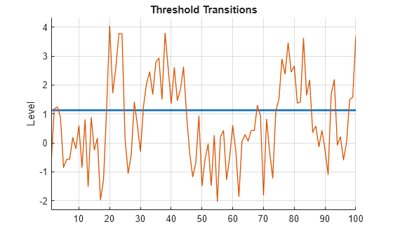
Create the following fully specified SETAR model for the DGP.
State 1: .
State 2: .
State 3:.
.
The system is in state 1 when , the system is in state 2 when , and the system is in state 3 otherwise.
t = [-3 3];
ttDGP = threshold(t);
constant1 = [-1; -4];
constant2 = [1; 4];
constant3 = [1; 4];
AR1 = [-0.5 0.1; 0.2 -0.75];
AR3 = [0.5 0.1; 0.2 0.75];
Sigma = [2 -1; -1 1];
mdl1DGP = varm(Constant=constant1,AR={AR1});
mdl2DGP = varm(Constant=constant2);
mdl3DGP = varm(Constant=constant3,AR={AR3});
mdlDGP = [mdl1DGP; mdl2DGP; mdl3DGP];
MdlDGP = tsVAR(ttDGP,mdlDGP,Covariance=Sigma);
Display a summary of the unestimated DGP.
summarize(MdlDGP)
Mdl =
  tsVAR with properties:

         Switch: [1×1 threshold]
      Submodels: [3×1 varm]
      NumStates: 3
      NumSeries: 2
     StateNames: ["1"    "2"    "3"]
    SeriesNames: ["1"    "2"]
     Covariance: [2×2 double]
summarize prints an object display.
Generate a random response path of length 1000 from the DGP. Specify that second response variable with a delay of 4 as the threshold variable.
rng(10) % For reproducibiliy
y = simulate(MdlDGP,1000,Index=2,Delay=4);
Create a partially specified threshold-switching model that has the same structure as the DGP, but specify the transition mid-level, submodel coefficients, and model-wide covariance as unknown for estimation.
tt = threshold([NaN; NaN]);
mdlar = varm(2,1);
mdlc = varm(2,0);
Mdl = tsVAR(tt,[mdlar; mdlc; mdlar],Covariance=nan(2));
Fully specify a threshold transition that has the same structure as tt, but set the mid-levels to -1 and 1.
t0 = [-1 1];
tt0 = threshold(t0);
Fit the threshold-switching model to the simulated series. Specify the threshold variable . Plot the loglikelihood after each iteration of the threshold search algorithm.
EstMdl = estimate(Mdl,tt0,y,IterationPlot=true,Index=2,Delay=4);
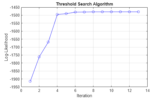
The plot displays the evolution of the loglikelihood as the estimation procedure searches for optimal levels. The procedure terminates when one of the stopping criteria is satisfied.
Display an estimation summary for state 3 only.
summarize(EstMdl,3)
Description
2-Dimensional VAR Submodel, State 3

Submodel
                           Estimate    StandardError    TStatistic      PValue
                           ________    _____________    __________    __________

    State 3 Constant(1)      1.1151       0.067611        16.494      4.0849e-61
    State 3 Constant(2)      3.8837       0.048939        79.357               0
    State 3 AR{1}(1,1)      0.53183       0.040671        13.077       4.486e-39
    State 3 AR{1}(2,1)      0.19554       0.029439         6.642       3.094e-11
    State 3 AR{1}(1,2)     0.097517       0.012623        7.7254      1.1149e-14
    State 3 AR{1}(2,2)      0.75156      0.0091369        82.255               0
Create a discrete threshold transition at mid-level 1.
ttDGP = threshold(1)
ttDGP =
  threshold with properties:

          Type: 'discrete'
        Levels: 1
         Rates: []
    StateNames: ["1"    "2"]
     NumStates: 2
Create the following fully specified self-exciting TAR (SETAR) model for the DGP.
State 1: .
State 2:
.
Specify the submodels by using arima.
mdl1DGP = arima(Constant=0);
mdl2DGP = arima(Constant=2);
mdlDGP = [mdl1DGP mdl2DGP];
Create a threshold-switching model for the DGP. Specify the model-wide innovations variance.
MdlDGP = tsVAR(ttDGP,mdlDGP,Covariance=1);
Generate a random response path of length 100 from the DGP. By default, simulate assumes a SETAR model with delay = 1. In other words, the threshold variable is .
rng(1) % For reproducibiliy
y = simulate(MdlDGP,100);
Create a partially specified threshold-switching model that has the same structure as the data-generating process, but specify the transition mid-level, submodel coefficients, and model-wide constant as unknown for estimation.
tt = threshold(NaN);
mdl1 = arima('Constant',NaN);
mdl2 = arima('Constant',NaN);
Mdl = tsVAR(tt,[mdl1,mdl2],'Covariance',NaN);
Fully specify a threshold transition that has the same structure as tt, but set the mid-level to 0.
tt0 = threshold(0);
Fit the model to the simulated path. By default, the model is self-exciting and the delay of the threshold variable is .
EstMdl = estimate(Mdl,tt0,y);
Return an estimation summary table.
results = summarize(EstMdl)
results=2×4 table
                           Estimate    StandardError    TStatistic      PValue
                           ________    _____________    __________    __________

    State 1 Constant(1)    -0.12774       0.13241        -0.96474        0.33467
    State 2 Constant(1)      2.1774       0.16829          12.939     2.7264e-38
results is a table containing estimates and inferences for all submodel coefficients.
Identify significant coefficient estimates.
results.Properties.RowNames(results.PValue < 0.05)
ans = 1×1 cell array
    {'State 2 Constant(1)'}
Input Arguments
Output Arguments
Algorithms
estimate searches over levels
and rates for estimated threshold transitions while solving a conditional least-squares
problem for submodel parameters, as described in [2]. The standard errors, loglikelihood, and
information criteria are conditional on optimal parameter values in the estimated threshold
transitions Mdl.Switch. In particular, standard errors do not account for
variation in estimated levels and rates.
References
Version History
Introduced in R2021b