Main Content

vratiotest

Variance ratio test for random walk

Description

example

h = vratiotest(y) returns the rejection decision h from conducting the variance ratio test for assessing whether the univariate time series y is a random walk.

example

[h,pValue,stat,cValue] = vratiotest(y) also returns the p-value pValue, test statistic stat, and critical value cValue of the test.

example

StatTbl = vratiotest(Tbl) returns the table StatTbl containing variables for the test results, statistics, and settings from conducting the variance ratio test on the last variable of the input table or timetable Tbl. To select a different variable in Tbl to test, use the DataVariable name-value argument.

example

[___] = vratiotest(___,Name=Value) specifies options using one or more name-value arguments in addition to any of the input argument combinations in previous syntaxes. vratiotest returns the output argument combination for the corresponding input arguments.

Some options control the number of tests to conduct. The following conditions apply when vratiotest conducts multiple tests:

  • vratiotest treats each test as separate from all other tests.

  • If you specify y, all outputs are vectors.

  • If you specify Tbl, each row of StatTbl contains the results of the corresponding test.

For example, vratiotest(Tbl,DataVariable="GDP",Alpha=0.025,IID=[false true]) conducts two tests, at a level of significance of 0.025, on the variable GDP of the table Tbl. The first test does not assume that the innovations series is iid and the second test assumes that the innovations series is iid.

example

[___,ratio] = vratiotest(___) additionally returns the variance ratios of each test ratio.

Examples

collapse all

Test whether a time series is a random walk using the default options of vratiotest. Input the time series data as a numeric vector.

Load the global large-cap equity indices data set, which contains daily closing prices during 1993–2003. Extract the closing prices of the S&P 500 series.

load Data_GlobalIdx1
dt = datetime(dates,ConvertFrom="datenum");
sp = DataTable.SP;
plot(dt,sp)
title("S&P 500 Price Series")

Figure contains an axes object. The axes object with title S&P 500 Price Series contains an object of type line.

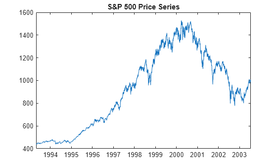
The first half of the series exhibits exponential growth.

Scale the series by applying the log transformation.

logsp = log(DataTable.SP);

The logsp series is in levels.

Assess the null hypothesis that the log series is a random walk by applying the variance ratio test. Use default options.

h = vratiotest(logsp)
h = logical
   0

h = 0 indicates that, at a 5% level of significance, the test fails to reject the null hypothesis that the series is a random walk.

Load the global large-cap equity indices data set, extract the closing prices of the S&P 500 price series, and apply the log transform to the series.

load Data_GlobalIdx1
logsp = log(DataTable.SP);

Assess the null hypothesis that the log series is a random walk by applying the variance ratio test. Return the test decision, p-value, test statistic, and critical value.

[h,pValue,stat,cValue] = vratiotest(logsp)
h = logical
   0

pValue = 0.7004
stat = 0.3847
cValue = 1.9600

Test whether a time series, which is one variable in a table, is a random walk using the default options.

Load the global large-cap equity indices data set. Convert the table DataTable to a timetable.

load Data_GlobalIdx1
dates = datetime(dates,ConvertFrom="datenum");
TT = table2timetable(DataTable,RowTimes=dates);

Apply the log transform to all series.

LTT = varfun(@log,TT(:,2:end));
LTT.Properties.VariableNames{end}
ans = 
'log_SP'

The last variable in the table is the log of the S&P 500 price series log_SP.

Assess the null hypothesis of the variance ratio test that the log of the S&P 500 price series is a random walk.

StatTbl = vratiotest(LTT)
StatTbl=1×7 table
                h      pValue      stat      cValue    Alpha    Period     IID 
              _____    _______    _______    ______    _____    ______    _____

    Test 1    false    0.70045    0.38471     1.96     0.05       2       false

vratiotest returns test results and settings in the table StatTbl, where variables correspond to test results (h, pValue, stat, and cValue) and settings (Alpha, Period, and IID), and rows correspond to individual tests (in this case, vratiotest conducts one test).

By default, vratiotest tests the last variable in the table. To select a variable from an input table to test, set the DataVariable option.

Test whether the S&P 500 series is a random walk using various step sizes, with and without the iid innovations assumption.

Load the global large-cap equity indices data set. Convert the table DataTable to a timetable and apply the log transform to all timetable variables.

load Data_GlobalIdx1
dates = datetime(dates,ConvertFrom="datenum");
TT = table2timetable(DataTable,RowTimes=dates);
LTT = varfun(@log,TT(:,2:end));

Plot the S&P 500 returns.

plot(diff(LTT.log_SP))
axis tight

Figure contains an axes object. The axes object contains an object of type line.

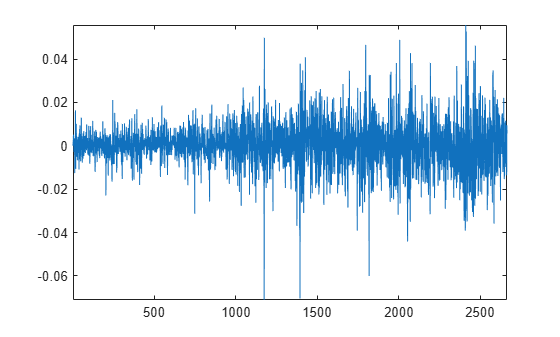
The plot indicates that the returns have possible conditional heteroscedasticity.

Conduct separate tests for whether the series is a random walk using periods 2, 4, and 8. For each period, conduct separate tests assuming the innovations are iid and without the assumption. Return the variance ratios of each test, and compute the first-order autocorrelation of the returns from the first ratio.

q = [2 4 8 2 4 8];
iid = logical([1 1 1 0 0 0]);
[StatTbl,ratio] = vratiotest(LTT,Period=q,IID=iid,DataVariable="log_SP")
StatTbl=6×7 table
                h       pValue       stat      cValue    Alpha    Period     IID 
              _____    ________    ________    ______    _____    ______    _____

    Test 1    false     0.56704     0.57242     1.96     0.05       2       true 
    Test 2    false     0.33073    -0.97265     1.96     0.05       4       true 
    Test 3    true     0.030933     -2.1579     1.96     0.05       8       true 
    Test 4    false     0.70045     0.38471     1.96     0.05       2       false
    Test 5    false     0.50788    -0.66214     1.96     0.05       4       false
    Test 6    false     0.13034     -1.5128     1.96     0.05       8       false

ratio = 6×1

    1.0111
    0.9647
    0.8763
    1.0111
    0.9647
    0.8763

rho1 = ratio(1) - 1 % First-order autocorrelation of returns
rho1 = 0.0111

StatTbl.h indicates that the test fails to reject that the series is a random walk at 5% level, except in the case where period = 8 and IID = true. This rejection is likely due to the test not accounting for the heteroscedasticity.

Input Arguments

collapse all

Univariate time series data in levels, specified as a numeric vector. Each element of y represents an observation.

Data Types: double

Time series data, specified as a table or timetable. Each row of Tbl is an observation.

Specify a single series (variable) to test by using the DataVariable argument. The selected variable must be numeric.

Note

  • vratiotest removes missing observations, represented by NaN values, from the input series.

  • vratiotest assumes that the specified input data is in levels. To convert a return series r to levels, define y(1) appropriately and let y = cumsum([y(1) r]).

Name-Value Arguments

Specify optional pairs of arguments as Name1=Value1,...,NameN=ValueN, where Name is the argument name and Value is the corresponding value. Name-value arguments must appear after other arguments, but the order of the pairs does not matter.

Before R2021a, use commas to separate each name and value, and enclose Name in quotes.

Example: vratiotest(Tbl,DataVariable="GDP",Alpha=0.025,IID=[false true]) conducts two tests, at a level of significance of 0.025, on the variable GDP of the table Tbl. The first test does not assume that the innovations series is iid and the second test assumes that the innovations series is iid.

Period q used to create overlapping return horizons for the variance ratio, specified as an integer that is greater than 1 and less T/2 or a vector of such integers, where T is the effective sample size of yt.

When Period = 2 (the default), the first-order autocorrelation of the returns is asymptotically equal to ratio − 1.

vratiotest conducts a separate test for each value in Period.

Example: Period=2:4 runs three tests; the first test sets Period to 2, the second test sets Period to 3, and the third test sets Period to 4.

Data Types: double

Flag for whether to assume the innovations are iid, specified as a value in this table or a vector of such values.

ValueDescription
false

Innovations are not iid; the alternative hypothesis is the innovations series εt is a correlated series.

Set false when the input series is a long-term macroeconomic or financial price series because often, for such series, the iid assumption is unreasonable and rejection of the random-walk null hypothesis is due to heteroscedasticity is uninteresting.

true

Innovations are iid; the alternative hypothesis is εt is a dependent or not identically distributed series (for example, heteroscedastic).

Set true to strengthen the random-walk null hypothesis.

vratiotest conducts a separate test for each value in IID.

Example: IID=true

Data Types: double

Nominal significance level for the hypothesis test, specified as a numeric scalar in the interval (0,1) or a numeric vector of such values.

vratiotest conducts a separate test for each value in Alpha.

Example: Alpha=[0.01 0.05] uses a level of significance of 0.01 for the first test, and then uses a level of significance of 0.05 for the second test.

Data Types: double

Variable in Tbl to test, specified as a string scalar or character vector containing a variable name in Tbl.Properties.VariableNames, or an integer or logical vector representing the index of a name. The selected variable must be numeric.

Example: DataVariable="GDP"

Example: DataVariable=[false true false false] or DataVariable=2 tests the second table variable.

Data Types: double | logical | char | string

Note

  • If you perform sequential testing using multiple values of q (Period), small-sample size distortions, beyond those that result from the asymptotic approximation of critical values, can result [2].

  • When vratiotest conducts multiple tests, the function applies all single settings (scalars or character vectors) to each test.

  • All vector-valued specifications that control the number of tests must have equal length.

  • If you specify the vector y and any value is a row vector, all outputs are row vectors.

Output Arguments

collapse all

Test rejection decisions, returned as a logical scalar or vector with length equal to the number of tests. vratiotest returns h when you supply the input y.

  • Values of 1 indicate rejection of the random-walk null hypothesis in favor of the alternative.

  • Values of 0 indicate failure to reject the random-walk null hypothesis.

Test statistic p-values, returned as a numeric scalar or vector with length equal to the number of tests. vratiotest returns pValue when you supply the input res.

p-values are standard normal probabilities.

Test statistics, returned as a numeric scalar or vector with length equal to the number of tests. vratiotest returns stat when you supply the input y.

Test statistics are asymptotically standard normal.

Critical values, returned as a numeric scalar or vector with length equal to the number of tests. vratiotest returns cValue when you supply the input y.

Critical values are for two-tail probabilities.

Test summary, returned as a table with variables for the outputs h, pValue, stat, and cValue, and with a row for each test. vratiotest returns StatTbl when you supply the input Tbl.

StatTbl contains variables for the test settings specified by Period, Alpha, and IID.

Variance ratios, returned as a numeric vector with length equal to the number of tests. Each ratio is the ratio of the following quantities:

  • The variance of the q-fold overlapping return horizon

  • q times the variance of the return series

For a random walk, the ratios are asymptotically equal to one. For a mean-reverting series, the ratios are less than one. For a mean-averting series, the ratios are greater than one.

More About

collapse all

Variance Ratio Test

The variance ratio test assesses the null hypothesis that a univariate time series yt is a random walk. The null model is

yt = c + yt–1 + εt,

where c is a drift constant and εt is an uncorrelated innovations series with zero mean.

  • When the innovations are not iid (the IID argument is false), the alternative is εt is a correlated series.

  • When innovations are iid (IID is true), the alternative is εt is either a dependent or not identically distributed series (for example, heteroscedastic).

The test statistic is based on a ratio of variance estimates of returns rt = ytyt−1 and period q (Period argument) return horizons t + … + rtq+1.

The variance ratio (ratio output) is for a test is

VAR(rt+...+rtq+1)qVAR(rt).

The horizon overlaps to increase the efficiency of the estimator and power of the test. Under either null hypothesis, an uncorrelated εt series implies that the period q variance is asymptotically equal to q times the period 1 variance. However, the variance of the ratio depends on the degree of heteroscedasticity, and, therefore, the variance of the ratio depends on the null hypothesis.

Rejection of the null hypothesis due to dependence of the innovations does not imply that the εt are correlated. If the innovations are dependent, nonlinear functions of εt can be correlated, regardless of whether εt are correlated. For example, if Cov(εt,εtk) = 0 for all k ≠ 0, a k ≠ 0 can exist such that Cov(εt2,εtk2) ≠ 0.

The test is two-tailed; therefore, the test rejects the random-walk null hypothesis when the test statistic is outside of the critical interval [−cValue,cValue]. Each tail outside of the critical interval has probability Alpha/2.

Tips

  • The test finds the largest integer n such that nq ≤ T – 1, where q is the vaule of the Period argument and T is the sample size. Then, the test discards the final (T–1) – nq observations. To include these final observations, remove the initial (T–1) – nq observations from the input series before you run the test.

References

[1] Campbell, J. Y., A. W. Lo, and A. C. MacKinlay. Chapter 12. “The Econometrics of Financial Markets.” Nonlinearities in Financial Data. Princeton, NJ: Princeton University Press, 1997.

[2] Cecchetti, S. G., and P. S. Lam. “Variance-Ratio Tests: Small-Sample Properties with an Application to International Output Data.” Journal of Business and Economic Statistics. Vol. 12, 1994, pp. 177–186.

[3] Cochrane, J. “How Big is the Random Walk in GNP?” Journal of Political Economy. Vol. 96, 1988, pp. 893–920.

[4] Faust, J. “When Are Variance Ratio Tests for Serial Dependence Optimal?” Econometrica. Vol. 60, 1992, pp. 1215–1226.

[5] Lo, A. W., and A. C. MacKinlay. “Stock Market Prices Do Not Follow Random Walks: Evidence from a Simple Specification Test.” Review of Financial Studies. Vol. 1, 1988, pp. 41–66.

[6] Lo, A. W., and A. C. MacKinlay. “The Size and Power of the Variance Ratio Test.” Journal of Econometrics. Vol. 40, 1989, pp. 203–238.

[7] Lo, A. W., and A. C. MacKinlay. A Non-Random Walk Down Wall St. Princeton, NJ: Princeton University Press, 2001.

Version History

Introduced in R2009b