Unit Root Nonstationarity
What Is a Unit Root Test?
A unit root process is a data-generating process whose first difference is stationary. In other words, a unit root process yt has the form
yt = yt–1 + stationary process.
A unit root test attempts to determine whether a given time series is consistent with a unit root process.
The next section gives more details of unit root processes, and suggests why it is important to detect them.
Modeling Unit Root Processes
There are two basic models for economic data with linear growth characteristics:
Trend-stationary process (TSP): yt = c + δt + stationary process
Unit root process, also called a difference-stationary process (DSP): Δyt = δ + stationary process
Here Δ is the differencing operator, Δyt = yt – yt–1 = (1 – L)yt, where L is the lag operator defined by Liyt = yt – i.
The processes are indistinguishable for finite data. In other words, there are both a TSP and a DSP that fit a finite data set arbitrarily well. However, the processes are distinguishable when restricted to a particular subclass of data-generating processes, such as AR(p) processes. After fitting a model to data, a unit root test checks if the AR(1) coefficient is 1.
There are two main reasons to distinguish between these types of processes:
Forecasting
A TSP and a DSP produce different forecasts. Basically, shocks to a TSP return to the trend line as time increases. In contrast, shocks to a DSP might be persistent over time.
For example, consider the simple trend-stationary model
and the difference-stationary model
In these models, and are independent innovation processes. For this example, the innovations are independent and distributed N(0,1).
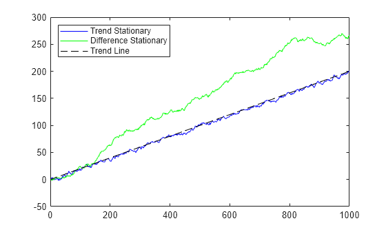
Both processes grow at rate 0.2. To calculate the growth rate for the TSP, which has a linear term , set . Then, solve the model for and .
The solution is , .
A plot for t = 1:1000 shows the TSP stays very close to the trend line, while the DSP has persistent deviations away from the trend line.
T = 1000;   % Sample size
t = (1:T)'; % Period vector
rng(5);     % For reproducibility

randm = randn(T,2); % Innovations
y = zeros(T,2);     % Columns of y are data series

% Build trend stationary series
y(:,1) = .02*t + randm(:,1);
for ii = 2:T
    y(ii,1) = y(ii,1) + y(ii-1,1)*.9;
end

% Build difference stationary series
y(:,2) = .2 + randm(:,2);
y(:,2) = cumsum(y(:,2));

figure
plot(y(:,1),'b')
hold on
plot(y(:,2),'g')
plot((1:T)*0.2,'k--')
legend('Trend Stationary','Difference Stationary',...
    'Trend Line','Location','NorthWest')
hold off
Forecasts based on the two series are different. To see this difference, plot the predicted behavior of the two series using varm, estimate, and forecast. The following plot shows the last 100 data points in the two series and predictions of the next 100 points, including confidence bounds.
AR = {[NaN 0; 0 NaN]}; % Independent response series
trend = [NaN; 0];      % Linear trend in first series only
Mdl = varm('AR',AR,'Trend',trend);

EstMdl = estimate(Mdl,y);
EstMdl.SeriesNames = ["Trend stationary" "Difference stationary"];

[ynew,ycov] = forecast(EstMdl,100,y);
% This generates predictions for 100 time steps

seY = sqrt(diag(EstMdl.Covariance))'; % Extract standard deviations of y
CIY = zeros([size(y) 2]);             % In-sample intervals
CIY(:,:,1) = y - seY;
CIY(:,:,2) = y + seY;

extractFSE = cellfun(@(x)sqrt(diag(x))',ycov,'UniformOutput',false);
seYNew = cell2mat(extractFSE);
CIYNew = zeros([size(ynew) 2]); % Forecast intervals
CIYNew(:,:,1) = ynew - seYNew;
CIYNew(:,:,2) = ynew + seYNew;

tx = (T-100:T+100);
hs = 1:2;
figure;
for j = 1:Mdl.NumSeries
    hs(j) = subplot(2,1,j);
    hold on;
    h1 = plot(tx,tx*0.2,'k--');
    axis tight;
    ha = gca;
    h2 = plot(tx,[y(end-100:end,j); ynew(:,j)]);
    h3 = plot(tx(1:101),squeeze(CIY(end-100:end,j,:)),'r:');
    plot(tx(102:end),squeeze(CIYNew(:,j,:)),'r:');
    h4 = fill([tx(102) ha.XLim([2 2]) tx(102)],ha.YLim([1 1 2 2]),[0.7 0.7 0.7],...
        'FaceAlpha',0.1,'EdgeColor','none');
    title(EstMdl.SeriesNames{j});
    hold off;
end
legend(hs(1),[h1 h2 h3(1) h4],...
    {'Trend','Process','Interval estimate','Forecast horizon'},'Location','Best');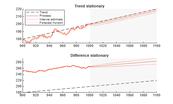
Examine the fitted parameters by passing the estimated model to summarize, and you find estimate did an excellent job.
The TSP has confidence intervals that do not grow with time, whereas the DSP has confidence intervals that grow. Furthermore, the TSP goes to the trend line quickly, while the DSP does not tend towards the trend line asymptotically.
Spurious Regression
The presence of unit roots can lead to false inferences in regressions between time series.
Suppose xt and yt are unit root processes with independent increments, such as random walks with drift
xt =
c1 +
xt–1 +
ε1(t)
yt
= c2 +
yt–1 +
ε2(t),
where εi(t) are independent innovations processes. Regressing y on x results, in general, in a nonzero regression coefficient, and significant coefficient of determination R2. This result holds despite xt and yt being independent random walks.
If both processes have trends (ci ≠ 0), there is a correlation between x and y because of their linear trends. However, even if the ci = 0, the presence of unit roots in the xt and yt processes yields correlation. For more information on spurious regression, see Granger and Newbold [1] and Time Series Regression IV: Spurious Regression.
Available Tests
There are four Econometrics Toolbox™ tests for unit roots. These functions test for the existence of a single unit root. When there are two or more unit roots, the results of these tests might not be valid.
Dickey-Fuller and Phillips-Perron Tests
adftest performs the augmented Dickey-Fuller
test. pptest performs the Phillips-Perron test. These
two classes of tests have a null hypothesis of a unit root process of the form
yt = yt–1 + c + δt + εt,
which the functions test against an alternative model
yt = γyt–1 + c + δt + εt,
where γ < 1. The null and alternative models for a Dickey-Fuller
test are like those for a Phillips-Perron test. The difference is
adftest extends the model with extra parameters accounting for
serial correlation among the innovations:
yt = c + δt + γyt – 1 + ϕ1Δyt – 1 + ϕ2Δyt – 2 +...+ ϕpΔyt – p + εt,
where
L is the lag operator: Lyt = yt–1.
Δ = 1 – L, so Δyt = yt – yt–1.
εt is the innovations process.
Phillips-Perron adjusts the test statistics to account for serial correlation.
There are three variants of both adftest and
pptest, corresponding to the following values of the
'model' parameter:
'AR'assumes c and δ, which appear in the preceding equations, are both0; the'AR'alternative has mean 0.'ARD'assumes δ is0. The'ARD'alternative has mean c/(1–γ).'TS'makes no assumption about c and δ.
For information on how to choose the appropriate value of 'model',
see Choose Models to Test.
KPSS Test
The KPSS test, kpsstest, is an inverse of the Phillips-Perron
test: it reverses the null and alternative hypotheses. The KPSS test uses the
model:
yt =
ct + δt +
ut,
with
ct =
ct–1 +
vt.
Here ut is a stationary process, and vt is an iid process with mean 0 and variance σ2. The null hypothesis is that σ2 = 0, so that the random walk term ct becomes a constant intercept. The alternative is σ2 > 0, which introduces the unit root in the random walk.
Variance Ratio Test
The variance ratio test, vratiotest, is based on the fact that the
variance of a random walk increases linearly with time. vratiotest
can also take into account heteroscedasticity, where the variance increases at a variable
rate with time. The test has a null hypotheses of a random walk:
Δyt = εt.
Testing for Unit Roots
Transform Data
Transform your time series to be approximately linear before testing for a unit root. If a series has exponential growth, take its logarithm. For example, GDP and consumer prices typically have exponential growth, so test their logarithms for unit roots.
If you want to transform your data to be stationary instead of approximately linear, unit root tests can help you determine whether to difference your data, or to subtract a linear trend. For a discussion of this topic, see What Is a Unit Root Test?
Choose Models to Test
For
adftestorpptest, choosemodelin as follows:If your data shows a linear trend, set
modelto'TS'.If your data shows no trend, but seem to have a nonzero mean, set
modelto'ARD'.If your data shows no trend and seem to have a zero mean, set
modelto'AR'(the default).
For
kpsstest, settrendtotrue(default) if the data shows a linear trend. Otherwise, settrendtofalse.For
vratiotest, setIIDtotrueif you want to test for independent, identically distributed innovations (no heteroscedasticity). Otherwise, leaveIIDat the default value,false. Linear trends do not affectvratiotest.
Determine Appropriate Lags
Setting appropriate lags depends on the test you use:
adftest— One method is to begin with a maximum lag, such as the one recommended by Schwert [2]. Then, test down by assessing the significance of the coefficient of the term at lag pmax. Schwert recommends a maximum lag ofwhere is the integer part of x. The usual t statistic is appropriate for testing the significance of coefficients, as reported in the
regoutput structure.Another method is to combine a measure of fit, such as SSR, with information criteria such as AIC, BIC, and HQC. These statistics also appear in the
regoutput structure. Ng and Perron [3] provide further guidelines.kpsstest— One method is to begin with few lags, and then evaluate the sensitivity of the results by adding more lags. For consistency of the Newey-West estimator, the number of lags must go to infinity as the sample size increases. Kwiatkowski et al. [4] suggest using a number of lags on the order of T1/2, where T is the sample size.For an example of choosing lags for
kpsstest, see Test Time Series Data for Unit Root.pptest— One method is to begin with few lags, and then evaluate the sensitivity of the results by adding more lags. Another method is to look at sample autocorrelations of yt – yt–1; slow rates of decay require more lags. The Newey-West estimator is consistent if the number of lags is O(T1/4), where T is the effective sample size, adjusted for lag and missing values. White and Domowitz [5] and Perron [6] provide further guidelines.For an example of choosing lags for
pptest, see Test Time Series Data for Unit Root.vratiotestdoes not use lags.
Conduct Unit Root Tests at Multiple Lags
Run multiple tests simultaneously by entering a vector of parameters for
lags, alpha, model, or
test. All vector parameters must have the same length. The test
expands any scalar parameter to the length of a vector parameter. For an example using
this technique, see Test Time Series Data for Unit Root.
References
[1] Granger, C. W. J., and P. Newbold. “Spurious Regressions in Econometrics.” Journal of Econometrics. Vol 2, 1974, pp. 111–120.
[2] Schwert, W. “Tests for Unit Roots: A Monte Carlo Investigation.” Journal of Business and Economic Statistics. Vol. 7, 1989, pp. 147–159.
[3] Ng, S., and P. Perron. “Unit Root Tests in ARMA Models with Data-Dependent Methods for the Selection of the Truncation Lag.” Journal of the American Statistical Association. Vol. 90, 1995, pp. 268–281.
[4] Kwiatkowski, D., P. C. B. Phillips, P. Schmidt, and Y. Shin. “Testing the Null Hypothesis of Stationarity against the Alternative of a Unit Root.” Journal of Econometrics. Vol. 54, 1992, pp. 159–178.
[5] White, H., and I. Domowitz. “Nonlinear Regression with Dependent Observations.” Econometrica. Vol. 52, 1984, pp. 143–162.
[6] Perron, P. “Trends and Random Walks in Macroeconomic Time Series: Further Evidence from a New Approach.” Journal of Economic Dynamics and Control. Vol. 12, 1988, pp. 297–332.
See Also
adftest | kpsstest | pptest | vratiotest