Asset Allocation Case Study
This example shows how to set up a basic asset allocation problem that uses mean-variance portfolio optimization with a Portfolio object to estimate efficient portfolios.
Step 1. Defining the portfolio problem.
Suppose that you want to manage an asset allocation fund with four asset classes: bonds, large-cap equities, small-cap equities, and emerging equities. The fund is long-only with no borrowing or leverage, should have no more than 85% of the portfolio in equities, and no more than 35% of the portfolio in emerging equities. The cost to trade the first three assets is 10 basis points annualized and the cost to trade emerging equities is four times higher. Finally, you want to ensure that average turnover is no more than 15%. To solve this problem, you will set up a basic mean-variance portfolio optimization problem and then slowly introduce the various constraints on the problem to get to a solution.
To set up the portfolio optimization problem, start with basic definitions of known quantities associated with the structure of this problem. Each asset class is assumed to have a tradeable asset with a real-time price. Such assets can be, for example, exchange-traded funds (ETFs). The initial portfolio with holdings in each asset that has a total of $7.5 million along with an additional cash position of $60,000. These basic quantities and the costs to trade are set up in the following variables with asset names in the cell array Asset, current prices in the vector Price, current portfolio holdings in the vector Holding, and transaction costs in the vector UnitCost.
To analyze this portfolio, you can set up a blotter in a table object to help track prices, holdings, weights, and so forth. In particular, you can compute the initial portfolio weights and maintain them in a new blotter field called InitPort.
Asset = { 'Bonds', 'Large-Cap Equities', 'Small-Cap Equities', 'Emerging Equities' };
Price = [ 52.4; 122.7; 35.2; 46.9 ];
Holding = [ 42938; 24449; 42612; 15991 ];
UnitCost = [ 0.001; 0.001; 0.001; 0.004 ];

Blotter = table('RowNames', Asset);
Blotter.Price = Price;
Blotter.InitHolding = Holding;
Wealth = sum(Blotter.Price .* Blotter.InitHolding);
Blotter.InitPort = (1/Wealth)*(Blotter.Price .* Blotter.InitHolding);
Blotter.UnitCost = UnitCost;
BlotterBlotter=4×4 table
Price InitHolding InitPort UnitCost
_____ ___________ ________ ________
Bonds 52.4 42938 0.3 0.001
Large-Cap Equities 122.7 24449 0.4 0.001
Small-Cap Equities 35.2 42612 0.2 0.001
Emerging Equities 46.9 15991 0.1 0.004
Step 2. Simulating asset prices.
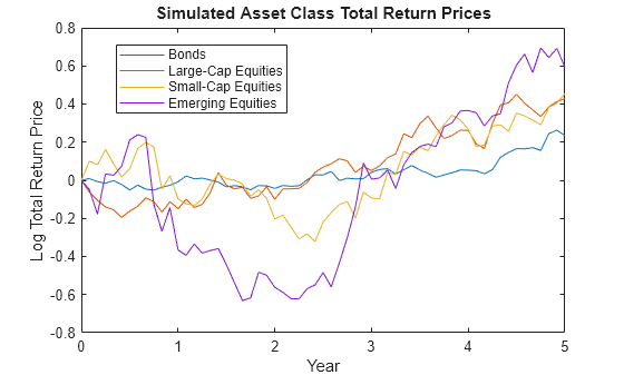
Since this is a hypothetical example, to simulate asset prices from a given mean and covariance of annual asset total returns for the asset classes, the portsim function is used to create asset returns with the desired mean and covariance. Specifically, portsim is used to simulate five years of monthly total returns and then plotted to show the log of the simulated total return prices.
The mean and covariance of annual asset total returns are maintained in the variables AssetMean and AssetCovar. The simulated asset total return prices (which are compounded total returns) are maintained in the variable Y. All initial asset total return prices are normalized to 1 in this example.
AssetMean = [ 0.05; 0.1; 0.12; 0.18 ];
AssetCovar = [ 0.0064 0.00408 0.00192 0;
    0.00408 0.0289 0.0204 0.0119;
    0.00192 0.0204 0.0576 0.0336;
    0 0.0119 0.0336 0.1225 ];

X = portsim(AssetMean'/12, AssetCovar/12, 60); % Monthly total returns for 5 years (60 months)
[Y, T] = ret2tick(X, [], 1/12);                % form total return prices.
plot(T, log(Y));
title('\bfSimulated Asset Class Total Return Prices');
xlabel('Year');
ylabel('Log Total Return Price');
legend(Asset,'Location','best');
Step 3. Setting up the Portfolio object.
To explore portfolios on the efficient frontier, set up a Portfolio object using these specifications:
Portfolio weights are nonnegative and sum to
1.Equity allocation is no more than 85% of the portfolio.
Emerging equity is no more than 35% of the portfolio.
These specifications are incorporated into the Portfolio object p in the following sequence of using functions that starts with using the Portfolio object.
The specification of the initial portfolio from
Blottergives the number of assets in your universe so you do not need to specify theNumAssetsproperty directly. Next, set up default constraints (long-only with a budget constraint). In addition, set up the group constraint that imposes an upper bound on equities in the portfolio (equities are identified in the group matrix with1's) and the upper bound constraint on emerging equities. Although you could have set the upper bound on emerging equities using thesetBoundsfunction, notice how theaddGroupsfunction is used to set up this constraint.To have a fully specified mean-variance portfolio optimization problem, you must specify the mean and covariance of asset returns. Since starting with these moments in the variables
AssetMeanandAssetCovar, you can use thesetAssetMomentsfunction to enter these variables into yourPortfolioobject (remember that you are assuming that your raw data are monthly returns which is why you divide your annual input moments by 12 to get monthly returns).Use the total return prices with the
estimateAssetMomentsfunction with a specification that your data inYare prices, and not returns, to estimate asset return moments for yourPortfolioobject.Although the returns in your
Portfolioobject are in units of monthly returns, and since subsequent costs are annualized, it is convenient to specify them as annualized total returns with this direct transformation of theAssetMeanandAssetCovarproperties of yourPortfolioobjectp.Display the
Portfolioobjectp.
p = Portfolio('Name', 'Asset Allocation Portfolio', ...
'AssetList', Asset, 'InitPort', Blotter.InitPort);

p = setDefaultConstraints(p);
p = setGroups(p, [ 0, 1, 1, 1 ], [], 0.85);
p = addGroups(p, [ 0, 0, 0, 1 ], [], 0.35);

p = setAssetMoments(p, AssetMean/12, AssetCovar/12);
p = estimateAssetMoments(p, Y, 'DataFormat', 'Prices');

p.AssetMean = 12*p.AssetMean;
p.AssetCovar = 12*p.AssetCovar;

display(p)
p =
  Portfolio with properties:

                       BuyCost: []
                      SellCost: []
                  RiskFreeRate: []
                     AssetMean: [4×1 double]
                    AssetCovar: [4×4 double]
                 TrackingError: []
                  TrackingPort: []
                      Turnover: []
                   BuyTurnover: []
                  SellTurnover: []
                          Name: 'Asset Allocation Portfolio'
                     NumAssets: 4
                     AssetList: {'Bonds'  'Large-Cap Equities'  'Small-Cap Equities'  'Emerging Equities'}
                      InitPort: [4×1 double]
                   AInequality: []
                   bInequality: []
                     AEquality: []
                     bEquality: []
                    LowerBound: [4×1 double]
                    UpperBound: []
                   LowerBudget: 1
                   UpperBudget: 1
                   GroupMatrix: [2×4 double]
                    LowerGroup: []
                    UpperGroup: [2×1 double]
                        GroupA: []
                        GroupB: []
                    LowerRatio: []
                    UpperRatio: []
                  MinNumAssets: []
                  MaxNumAssets: []
    ConditionalBudgetThreshold: []
        ConditionalUpperBudget: []
                     BoundType: [4×1 categorical]
Step 4. Validate the portfolio problem.
An important step in portfolio optimization is to validate that the portfolio problem is feasible and the main test is to ensure that the set of portfolios is nonempty and bounded. Use the estimateBounds function to determine the bounds for the portfolio set. In this case, since both lb and ub are finite, the set is bounded.
[lb, ub] = estimateBounds(p);
display([lb, ub])
    0.1500    1.0000
         0    0.8500
         0    0.8500
         0    0.3500
Step 5. Plotting the efficient frontier.
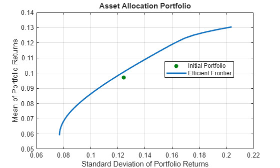
Given the constructed Portfolio object, use the plotFrontier function to view the efficient frontier. Instead of using the default of 10 portfolios along the frontier, you can display the frontier with 40 portfolios. Notice gross efficient portfolio returns fall between approximately 6% and 16% per years.
plotFrontier(p, 40)

Step 6. Evaluating gross vs. net portfolio returns.
The Portfolio object p does not include transaction costs so that the portfolio optimization problem specified in p uses gross portfolio return as the return proxy. To handle net returns, create a second Portfolio object q that includes transaction costs.
q = setCosts(p, UnitCost, UnitCost);
display(q)
q =
  Portfolio with properties:

                       BuyCost: [4×1 double]
                      SellCost: [4×1 double]
                  RiskFreeRate: []
                     AssetMean: [4×1 double]
                    AssetCovar: [4×4 double]
                 TrackingError: []
                  TrackingPort: []
                      Turnover: []
                   BuyTurnover: []
                  SellTurnover: []
                          Name: 'Asset Allocation Portfolio'
                     NumAssets: 4
                     AssetList: {'Bonds'  'Large-Cap Equities'  'Small-Cap Equities'  'Emerging Equities'}
                      InitPort: [4×1 double]
                   AInequality: []
                   bInequality: []
                     AEquality: []
                     bEquality: []
                    LowerBound: [4×1 double]
                    UpperBound: []
                   LowerBudget: 1
                   UpperBudget: 1
                   GroupMatrix: [2×4 double]
                    LowerGroup: []
                    UpperGroup: [2×1 double]
                        GroupA: []
                        GroupB: []
                    LowerRatio: []
                    UpperRatio: []
                  MinNumAssets: []
                  MaxNumAssets: []
    ConditionalBudgetThreshold: []
        ConditionalUpperBudget: []
                     BoundType: [4×1 categorical]
Step 7. Analyzing descriptive properties of the Portfolio structures.
To be more concrete about the ranges of efficient portfolio returns and risks, use the estimateFrontierLimits function to obtain portfolios at the endpoints of the efficient frontier. Given these portfolios, compute their moments using the estimatePortMoments function. The following code generates a table that lists the risk and return of the initial portfolio as well as the gross and net moments of portfolio returns for the portfolios at the endpoints of the efficient frontier:
[prsk0, pret0] = estimatePortMoments(p, p.InitPort);

pret = estimatePortReturn(p, p.estimateFrontierLimits);
qret = estimatePortReturn(q, q.estimateFrontierLimits);

displayReturns(pret0, pret, qret)
Annualized Portfolio Returns ...
                                    Gross       Net
Initial Portfolio Return             9.70 %    9.70 %
Minimum Efficient Portfolio Return   5.90 %    5.77 %
Maximum Efficient Portfolio Return  13.05 %   12.86 %
The results show that the cost to trade ranges from 14 to 19 basis points to get from the current portfolio to the efficient portfolios at the endpoints of the efficient frontier (these costs are the difference between gross and net portfolio returns.) In addition, notice that the maximum efficient portfolio return (13%) is less than the maximum asset return (18%) due to the constraints on equity allocations.
Step 8. Obtaining a Portfolio at the specified return level on the efficient frontier.
A common approach to select efficient portfolios is to pick a portfolio that has a desired fraction of the range of expected portfolio returns. To obtain the portfolio that is 30% of the range from the minimum to maximum return on the efficient frontier, obtain the range of net returns in qret using the Portfolio object q and interpolate to obtain a 30% level with the interp1 function to obtain a portfolio qwgt.
Level = 0.3;

qret = estimatePortReturn(q, q.estimateFrontierLimits);
qwgt = estimateFrontierByReturn(q, interp1([0, 1], qret, Level));
[qrsk, qret] = estimatePortMoments(q, qwgt);

displayReturnLevel(Level, qret, qrsk);
Portfolio at 30% return level on efficient frontier ...
    Return       Risk
      7.90       9.09
display(qwgt)
qwgt = 4×1

    0.6252
    0.1856
    0.0695
    0.1198
The target portfolio that is 30% of the range from minimum to maximum net returns has a return of 7.9% and a risk of 9.1%.
Step 9. Obtaining a Portfolio at the specified risk levels on the efficient frontier.
Although you could accept this result, suppose that you want to target values for portfolio risk. Specifically, suppose that you have a conservative target risk of 10%, a moderate target risk of 15%, and an aggressive target risk of 20% and you want to obtain portfolios that satisfy each risk target. Use the estimateFrontierByRisk function to obtain targeted risks specified in the variable TargetRisk. The resultant three efficient portfolios are obtained in qwgt.
TargetRisk = [ 0.10; 0.15; 0.20 ];
qwgt = estimateFrontierByRisk(q, TargetRisk);
display(qwgt)
qwgt = 4×3

    0.5407    0.2020    0.1500
    0.2332    0.4000    0.0318
    0.0788    0.1280    0.4682
    0.1474    0.2700    0.3500
Use the estimatePortRisk function to compute the portfolio risks for the three portfolios to confirm that the target risks have been attained:
display(estimatePortRisk(q, qwgt))
    0.1000
    0.1500
    0.2000
Suppose that you want to shift from the current portfolio to the moderate portfolio. You can estimate the purchases and sales to get to this portfolio:
[qwgt, qbuy, qsell] = estimateFrontierByRisk(q, 0.15);
If you average the purchases and sales for this portfolio, you can see that the average turnover is 17%, which is greater than the target of 15%:
disp(sum(qbuy + qsell)/2)
0.1700
Since you also want to ensure that average turnover is no more than 15%, you can add the average turnover constraint to the Portfolio object using setTurnover:
q = setTurnover(q, 0.15);
[qwgt, qbuy, qsell] = estimateFrontierByRisk(q, 0.15);
You can enter the estimated efficient portfolio with purchases and sales into the Blotter:
qbuy(abs(qbuy) < 1.0e-5) = 0;
qsell(abs(qsell) < 1.0e-5) = 0;  % Zero out near 0 trade weights.

Blotter.Port = qwgt;
Blotter.Buy = qbuy;
Blotter.Sell = qsell;

display(Blotter)Blotter=4×7 table
Price InitHolding InitPort UnitCost Port Buy Sell
_____ ___________ ________ ________ _______ ____ ________
Bonds 52.4 42938 0.3 0.001 0.18787 0 0.11213
Large-Cap Equities 122.7 24449 0.4 0.001 0.4 0 0
Small-Cap Equities 35.2 42612 0.2 0.001 0.16213 0 0.037871
Emerging Equities 46.9 15991 0.1 0.004 0.25 0.15 0
The Buy and Sell elements of the Blotter are changes in portfolio weights that must be converted into changes in portfolio holdings to determine the trades. Since you are working with net portfolio returns, you must first compute the cost to trade from your initial portfolio to the new portfolio. This is accomplished as follows:
TotalCost = Wealth * sum(Blotter.UnitCost .* (Blotter.Buy + Blotter.Sell))
TotalCost =
5.6248e+03
The cost to trade is $5,625, so that, in general, you would have to adjust your initial wealth accordingly before setting up your new portfolio weights. However, to keep the analysis simple, note that you have sufficient cash ($60,0000) set aside to pay the trading costs and that you will not touch the cash position to build up any positions in your portfolio. Thus, you can populate your blotter with the new portfolio holdings and the trades to get to the new portfolio without making any changes in your total invested wealth. First, compute the portfolio holding:
Blotter.Holding = Wealth * (Blotter.Port ./ Blotter.Price);
Compute number of shares to Buy and Sell in your Blotter:
Blotter.BuyShare = Wealth * (Blotter.Buy ./ Blotter.Price);
Blotter.SellShare = Wealth * (Blotter.Sell ./ Blotter.Price);
Notice how you used an ad hoc truncation rule to obtain unit numbers of shares to buy and sell. Clean up the Blotter by removing the unit costs and the buy and sell portfolio weights:
Blotter.Buy = [];
Blotter.Sell = [];
Blotter.UnitCost = [];
Step 10. Displaying the final results.
The final result is a blotter that contains proposed trades to get from your current portfolio to a moderate-risk portfolio. To make the trade, you would need to sell 16,049 shares of your bond asset and 8,069 shares of your small-cap equity asset and would need to purchase 23,986 shares of your emerging equities asset.
display(Blotter)
Blotter=4×7 table
                          Price    InitHolding    InitPort     Port      Holding    BuyShare    SellShare
                          _____    ___________    ________    _______    _______    ________    _________

    Bonds                  52.4       42938         0.3       0.18787     26889          0        16049
    Large-Cap Equities    122.7       24449         0.4           0.4     24449          0            0
    Small-Cap Equities     35.2       42612         0.2       0.16213     34543          0       8068.8
    Emerging Equities      46.9       15991         0.1          0.25     39977      23986            0
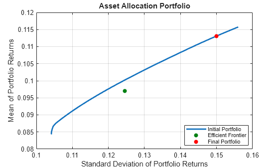
The final plot uses the plotFrontier function to display the efficient frontier and the initial portfolio for the fully specified portfolio optimization problem. It also adds the location of the moderate-risk or final portfolio on the efficient frontier.
plotFrontier(q, 40);
hold on
scatter(estimatePortRisk(q, qwgt), estimatePortReturn(q, qwgt), 'filled', 'r');
h = legend('Initial Portfolio', 'Efficient Frontier', 'Final Portfolio', 'location', 'best');
set(h, 'Fontsize', 8);
hold off

Local Functions
function displayReturns(pret0, pret, qret)
fprintf('Annualized Portfolio Returns ...\n');
fprintf('                                   %6s    %6s\n','Gross','Net');
fprintf('Initial Portfolio Return           %6.2f %%  %6.2f %%n',100*pret0,100*pret0);
fprintf('Minimum Efficient Portfolio Return %6.2f %%  %6.2f %%n',100*pret(1),100*qret(1));
fprintf('Maximum Efficient Portfolio Return %6.2f %%  %6.2f %%n',100*pret(2),100*qret(2));
end

function displayReturnLevel(Level, qret, qrsk)
fprintf('Portfolio at %g%% return level on efficient frontier ...\n',100*Level);
fprintf('%10s %10s\n','Return','Risk');
fprintf('%10.2f %10.2f\n',100*qret,100*qrsk);
end
See Also
Portfolio | setBounds | addGroups | setAssetMoments | estimateAssetMoments | estimateBounds | plotFrontier | estimateFrontierLimits | estimateFrontierByRisk | estimatePortRisk
Topics
- Creating the Portfolio Object
- Working with Portfolio Constraints Using Defaults
- Validate the Portfolio Problem for Portfolio Object
- Estimate Efficient Portfolios for Entire Efficient Frontier for Portfolio Object
- Estimate Efficient Frontiers for Portfolio Object
- Postprocessing Results to Set Up Tradable Portfolios
- Portfolio Optimization with Semicontinuous and Cardinality Constraints
- Black-Litterman Portfolio Optimization Using Financial Toolbox
- Portfolio Optimization Against a Benchmark
- Portfolio Optimization Examples Using Financial Toolbox
- Portfolio Analysis with Turnover Constraints
- Leverage in Portfolio Optimization with a Risk-Free Asset
- Black-Litterman Portfolio Optimization Using Financial Toolbox
- Portfolio Optimization Using Factor Models
- Portfolio Optimization Using Social Performance Measure
- Diversify Portfolios Using Custom Objective
- Portfolio Object
- Portfolio Optimization Theory
- Portfolio Object Workflow