interp1
1-D data interpolation (table lookup)
Syntax
Description
vq = interp1(x,v,xq)interp1 uses linear interpolation. Vector
x contains the sample points, and v
contains the corresponding values, v(x).
Vector xq contains the coordinates of the query
points.
If you have multiple sets of data that are sampled at the same point
coordinates, then you can pass v as an array. Each column of
array v contains a different set of 1-D sample values.
vq = interp1(x,v,xq,method,extrapolation)x. Set extrapolation to
'extrap' when you want to use the
method algorithm for extrapolation. Alternatively, you
can specify a scalar value, in which case, interp1 returns
that value for all points outside the domain of x.
vq = interp1(v,xq)1 to n, where n
depends on the shape of v:
When v is a vector, the default points are
1:length(v).When v is an array, the default points are
1:size(v,1).
Use this syntax when you are not concerned about the absolute distances between points.
vq = interp1(v,xq,method,extrapolation)
pp = interp1(x,v,method,'pp')method algorithm.
Note
This syntax is not recommended. Use griddedInterpolant
instead.
Examples
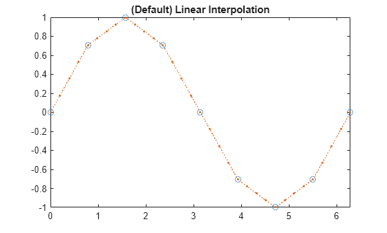
Define the sample points, x, and corresponding sample values, v.
x = 0:pi/4:2*pi;
v = sin(x);
Define the query points to be a finer sampling over the range of x.
xq = 0:pi/16:2*pi;
Interpolate the function at the query points and plot the result.
figure
vq1 = interp1(x,v,xq);
plot(x,v,'o',xq,vq1,':.');
xlim([0 2*pi]);
title('(Default) Linear Interpolation');
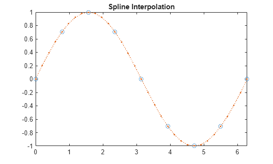
Now evaluate v at the same points using the 'spline' method.
figure
vq2 = interp1(x,v,xq,'spline');
plot(x,v,'o',xq,vq2,':.');
xlim([0 2*pi]);
title('Spline Interpolation');
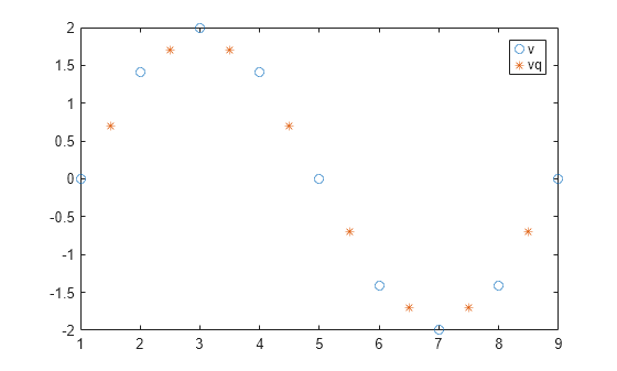
Define a set of function values.
v = [0 1.41 2 1.41 0 -1.41 -2 -1.41 0];
Define a set of query points that fall between the default points, 1:9. In this case, the default points are 1:9 because v contains 9 values.
xq = 1.5:8.5;
Evaluate v at xq.
vq = interp1(v,xq);
Plot the result.
figure
plot((1:9),v,'o',xq,vq,'*');
legend('v','vq');
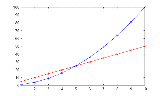
Define a set of sample points.
x = 1:10;
Define the values of the function, , at the sample points.
v = (5*x)+(x.^2*1i);
Define the query points to be a finer sampling over the range of x.
xq = 1:0.25:10;
Interpolate v at the query points.
vq = interp1(x,v,xq);
Plot the real part of the result in red and the imaginary part in blue.
figure
plot(x,real(v),'*r',xq,real(vq),'-r');
hold on
plot(x,imag(v),'*b',xq,imag(vq),'-b');
Interpolate time-stamped data points.
Consider a data set containing temperature readings that are measured every four hours. Create a table with one day's worth of data and plot the data.
x = (datetime(2016,1,1):hours(4):datetime(2016,1,2))';
x.Format = 'MMM dd, HH:mm';
T = [31 25 24 41 43 33 31]';
WeatherData = table(x,T,'VariableNames',{'Time','Temperature'})
WeatherData=7×2 table
        Time         Temperature
    _____________    ___________

    Jan 01, 00:00        31
    Jan 01, 04:00        25
    Jan 01, 08:00        24
    Jan 01, 12:00        41
    Jan 01, 16:00        43
    Jan 01, 20:00        33
    Jan 02, 00:00        31
plot(WeatherData.Time, WeatherData.Temperature, 'o')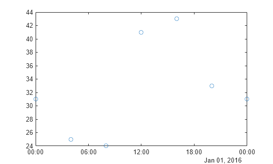
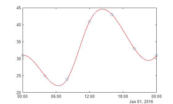
Interpolate the data set to predict the temperature reading during each minute of the day. Since the data is periodic, use the 'spline' interpolation method.
xq = (datetime(2016,1,1):minutes(1):datetime(2016,1,2))';
V = interp1(WeatherData.Time, WeatherData.Temperature, xq, 'spline');
Plot the interpolated points.
hold on
plot(xq,V,'r')
Define the sample points, x, and corresponding sample values, v.
x = [1 2 3 4 5];
v = [12 16 31 10 6];
Specify the query points, xq, that extend beyond the domain of x.
xq = [0 0.5 1.5 5.5 6];
Evaluate v at xq using the 'pchip' method.
vq1 = interp1(x,v,xq,'pchip')vq1 = 1×5
19.3684 13.6316 13.2105 7.4800 12.5600
Next, evaluate v at xq using the 'linear' method.
vq2 = interp1(x,v,xq,'linear')vq2 = 1×5
NaN NaN 14 NaN NaN
Now, use the 'linear' method with the 'extrap' option.
vq3 = interp1(x,v,xq,'linear','extrap')
vq3 = 1×5

     8    10    14     4     2
'pchip' extrapolates by default, but 'linear' does not.
Define the sample points, x, and corresponding sample values, v.
x = [-3 -2 -1 0 1 2 3];
v = 3*x.^2;
Specify the query points, xq, that extend beyond the domain of x.
xq = [-4 -2.5 -0.5 0.5 2.5 4];
Now evaluate v at xq using the 'pchip' method and assign any values outside the domain of x to the value, 27.
vq = interp1(x,v,xq,'pchip',27)vq = 1×6
27.0000 18.6562 0.9375 0.9375 18.6562 27.0000
Define the sample points.
x = (-5:5)';
Sample three different parabolic functions at the points defined in x.
v1 = x.^2;
v2 = 2*x.^2 + 2;
v3 = 3*x.^2 + 4;
Create matrix v, whose columns are the vectors, v1, v2, and v3.
v = [v1 v2 v3];
Define a set of query points, xq, to be a finer sampling over the range of x.
xq = -5:0.1:5;
Evaluate all three functions at xq and plot the results.
vq = interp1(x,v,xq,'pchip');
figure
plot(x,v,'o',xq,vq);

h = gca;
h.XTick = -5:5;
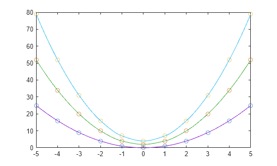
The circles in the plot represent v, and the solid lines represent vq.
Input Arguments
Output Arguments
More About
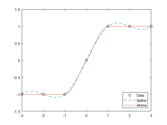
The Akima algorithm for one-dimensional interpolation, described in [1] and [2], performs cubic interpolation to produce piecewise polynomials with continuous first-order derivatives (C1). The algorithm preserves the slope and avoids undulations in flat regions. A flat region occurs whenever there are three or more consecutive collinear points, which the algorithm connects with a straight line. To ensure that the region between two data points is flat, insert an additional data point between those two points.
When two flat regions with different slopes meet, the modification made to the original Akima algorithm gives more weight to the side where the slope is closer to zero. This modification gives priority to the side that is closer to horizontal, which is more intuitive and avoids the overshoot. (The original Akima algorithm gives equal weights to the points on both sides, thus evenly dividing the undulation.)
The spline algorithm, on the other hand, performs cubic interpolation to produce piecewise polynomials with continuous second-order derivatives (C2). The result is comparable to a regular polynomial interpolation, but is less susceptible to heavy oscillation between data points for high degrees. Still, this method can be susceptible to overshoots and oscillations between data points.
Compared to the spline algorithm, the Akima algorithm produces fewer undulations and is better suited to deal with quick changes between flat regions. This difference is illustrated below using test data that connects multiple flat regions.
References
[1] Akima, Hiroshi. "A new method of interpolation and smooth curve fitting based on local procedures." Journal of the ACM (JACM) , 17.4, 1970, pp. 589-602.
[2] Akima, Hiroshi. "A method of bivariate interpolation and smooth surface fitting based on local procedures." Communications of the ACM , 17.1, 1974, pp. 18-20.