Hedge Options Using Reinforcement Learning Toolbox
This example shows how to outperform the traditional BSM approach using an optimal option hedging policy.
Option Modeling Using Black-Scholes-Merton Model
The Black-Scholes-Merton (BSM) model, which earned its creators a Nobel Prize in Economics in 1997, provides a modeling framework for pricing and analyzing financial derivatives or options. Options are financial instruments that derive their value from a particular underlying asset. The concept of dynamic hedging is fundamental to the BSM model. Dynamic hedging is the idea that, by continuously buying and selling shares in the relevant underlying asset, you can hedge the risk of the derivative instrument such that the risk is zero. This "risk-neutral" pricing framework is used to derive pricing formulae for many different financial instruments.
The simplest financial derivative is a European call option, which provides the buyer with the right, but not the obligation, to buy the underlying asset at a previously specified value (strike price) at a previously specified time (maturity).
You can use a BSM model to price a European call option. The BSM model makes the following simplifying assumptions:
The behavior of the underlying asset is defined by geometric Brownian motion (GBM).
There are no transaction costs.
Volatility is constant.
The BSM dynamic hedging strategy is also called "delta-hedging," after the quantity Delta, which is the sensitivity of the option with respect to the underlying asset. In an environment that meets the previously stated BSM assumptions, using a delta-hedging strategy is an optimal approach to hedging an option. However, it is well-known that in an environment with transaction costs, the use of the BSM model leads to an inefficient hedging strategy. The goal of this example is to use Reinforcement Learning Toolbox™ to learn a strategy that outperforms the BSM hedging strategy, in the presence of transaction costs.
The goal of reinforcement learning (RL) is to train an agent to complete a task within an unknown environment. The agent receives observations and a reward from the environment and sends actions to the environment. The reward is a measure of how successful an action is with respect to completing the task goal.
The agent contains two components: a policy and a learning algorithm.
The policy is a mapping that selects actions based on the observations from the environment. Typically, the policy is a function approximator with tunable parameters, such as a deep neural network.
The learning algorithm continuously updates the policy parameters based on the actions, observations, and reward. The goal of the learning algorithm is to find an optimal policy that maximizes the cumulative reward received during the task.
In other words, reinforcement learning involves an agent learning the optimal behavior through repeated trial-and-error interactions with the environment without human involvement. For more information on reinforcement learning, see What Is Reinforcement Learning? (Reinforcement Learning Toolbox).
Cao [2] describes the setup for reinforcement learning as:
is the state at time .
is the action taken at .
is the resulting reward at time .
The aim of reinforcement learning is to maximize expected future rewards. In this financial application of reinforcement learning, maximizing expected rewards is learning a delta-hedging strategy as an optimal approach to hedging a European call option.
This example follows the framework outlined in Cao [2]. Specifically, an accounting profit and loss (P&L) formulation from that paper is used to set up the reinforcement learning problem and a deep deterministic policy gradient (DDPG) agent is used. This example does not exactly reproduce the approach from [2] because Cao et. al. recommend a Q-learning approach with two separate Q-functions (one for the hedging cost and one for the expected square of the hedging cost), but this example uses instead a simplified reward function.
Define Training Parameters
Next, specify an at-the-money option with three months to maturity is hedged. For simplicity, both the interest rate and dividend yield are set to 0.
% Option parameters
Strike = 100;
Maturity = 21*3/250;

% Asset parameters
SpotPrice = 100;
ExpVol = .2;
ExpReturn = .05;

% Simulation parameters
rfRate = 0;
dT = 1/250;
nSteps = Maturity/dT;
nTrials = 5000;

% Transacation cost and cost function parameters
c = 1.5;
kappa = .01;
InitPosition = 0;

% Set the random generator seed for reproducibility.
rng(3)
Define Environment
In this section, you define the action and observation parameters, actInfo and obsInfo. The agent action is the current hedge value which can range between 0 and 1. There are three variables in the agent observation:
Moneyness (ratio of the spot price to the strike price)
Time to maturity
Position or amount of the underlying asset that is held
ObservationInfo             = rlNumericSpec([3 1],'LowerLimit',0,'UpperLimit',[10 Maturity 1]');
ObservationInfo.Name        = 'Hedging State';
ObservationInfo.Description = ['Moneyness', 'TimeToMaturity','Position'];

ActionInfo = rlNumericSpec([1 1],'LowerLimit',0,'UpperLimit',1);
ActionInfo.Name = 'Hedge';
Define Reward
From Cao [2], the accounting P&L formulation and rewards (negative costs) are
+ ( - ) -
where
A final reward at the last time step liquidates the hedge that is
In this implementation, the reward () is penalized by the square of the reward multiplied by a constant to punish large swings in the value of the hedged position:
The reward is defined in stepFcn which is called at each step of the simulation.
env = rlFunctionEnv(ObservationInfo,ActionInfo, ...
    @(Hedge, LoggedSignals) stepFcn(Hedge,LoggedSignals,rfRate,ExpVol,dT,Strike,ExpReturn,c,kappa), ...
    @() resetFcn(SpotPrice/Strike,Maturity,InitPosition));

obsInfo = getObservationInfo(env);
actInfo = getActionInfo(env);
Create Environment Interface for RL Agent
Create the DDPG agent using rlDDPGAgent (Reinforcement Learning Toolbox). While it is possible to create custom actor and critic networks, this example uses the default networks.
initOpts = rlAgentInitializationOptions('NumHiddenUnit',64);
criticOpts = rlOptimizerOptions("LearnRate",1e-4);
actorOpts = rlOptimizerOptions("LearnRate",1e-4);

agentOptions = rlDDPGAgentOptions(...
    "ActorOptimizerOptions",actorOpts, ...
    "CriticOptimizerOptions",criticOpts, ...
    "DiscountFactor",.9995, ...
    "TargetSmoothFactor",5e-4);
agent = rlDDPGAgent(obsInfo,actInfo,initOpts,agentOptions);
Visualize Actor and Critic Networks
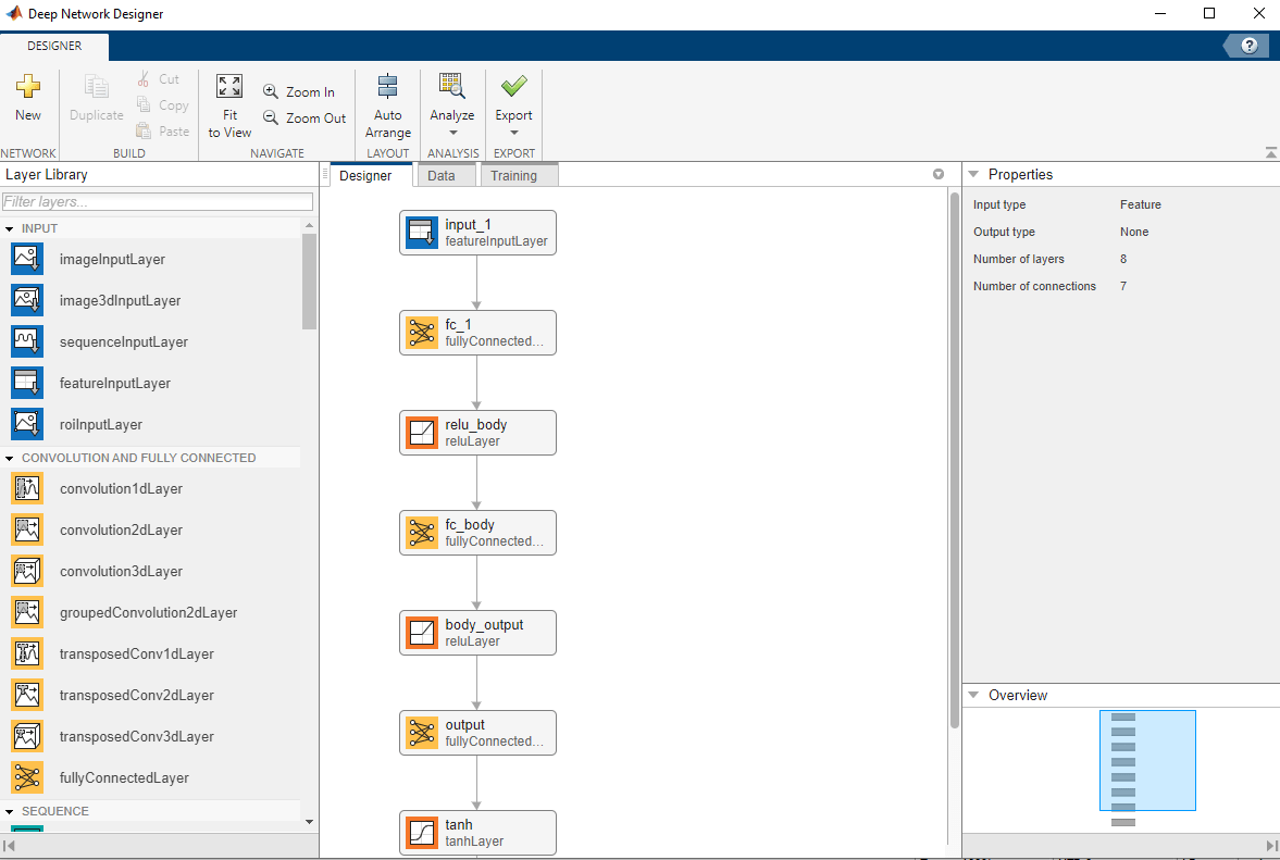
Visualize the actor and critic networks using the Deep Network Designer.
deepNetworkDesigner(getModel(getActor(agent)))

Train Agent
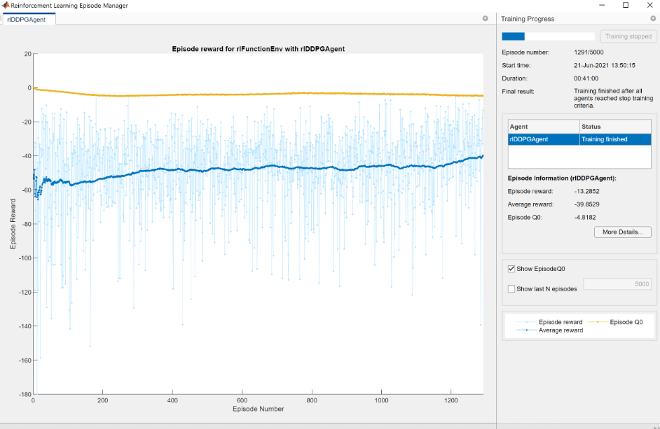
Train the agent using the train (Reinforcement Learning Toolbox) function.
trainOpts = rlTrainingOptions( ...
    'MaxEpisodes', nTrials, ...
    'MaxStepsPerEpisode',nSteps, ...
    'Verbose', false, ...
    'ScoreAveragingWindowLength',200,...
    'StopTrainingCriteria',"AverageReward", ...
    'StopTrainingValue',-40, ...
    'StopOnError',"on", ...
    "UseParallel",false);

doTraining = false;
if doTraining
    % Train the agent.
    trainingStats = train(agent,env,trainOpts);
else
    % Load the pretrained agent for the example.
    load('DeepHedgingDDPG.mat','agent')
end
To avoid waiting for the training, load pretrained networks by setting the doTraining flag to false. If you set doTraining to true, the Reinforcement Learning Episode Manager displays the training progress.

Validate Agent
Use the Financial Toolbox™ functions blsdelta and blsprice for a conventional approach to calculate the price as a European call option. When comparing the conventional approach to the RL approach, the results are similar to the findings of Cao [2] in Exhibit 4. This example demonstrates that the RL approach significantly reduces hedging costs.
% Simulation parameters
nTrials = 1000;

policy_BSM = @(mR,TTM,Pos) blsdelta(mR,1,rfRate,max(TTM,eps),ExpVol);

policy_RL = @(mR,TTM,Pos) arrayfun(@(mR,TTM,Pos) cell2mat(getAction(agent,[mR TTM Pos]')),mR,TTM,Pos);

OptionPrice = blsprice(SpotPrice,Strike,rfRate,Maturity,ExpVol);

Costs_BSM = computeCosts(policy_BSM,nTrials,nSteps,SpotPrice,Strike,Maturity,rfRate,ExpVol,InitPosition,dT,ExpReturn,kappa);
Costs_RL = computeCosts(policy_RL,nTrials,nSteps,SpotPrice,Strike,Maturity,rfRate,ExpVol,InitPosition,dT,ExpReturn,kappa);
HedgeComp = table(100*[-mean(Costs_BSM) std(Costs_BSM)]'/OptionPrice, ...
    100*[-mean(Costs_RL) std(Costs_RL)]'/OptionPrice, ...
    'RowNames',["Average Hedge Cost (% of Option Price)","STD Hedge Cost (% of Option Price)"], ...
    'VariableNames',["BSM","RL"]);
disp(HedgeComp)
                                               BSM        RL
                                              ______    ______

    Average Hedge Cost (% of Option Price)    91.259    47.022
    STD Hedge Cost (% of Option Price)        35.712    68.119
The following histogram shows the range of different hedging costs for both approaches. The RL approach performs better, but with a larger variance than the BSM approach. The RL approach in this example would likely benefit from the two Q-function approach that Cao [2] discusses and implements.
figure
numBins = 10;
histogram(-Costs_RL,numBins,'FaceColor','r','FaceAlpha',.5)
hold on
histogram(-Costs_BSM,numBins,'FaceColor','b','FaceAlpha',.5)
xlabel('Hedging Costs')
ylabel('Number of Trials')
title('RL Hedge Costs vs. BLS Hedge Costs')
legend('RL Hedge','Theoretical BLS Delta','location','best')

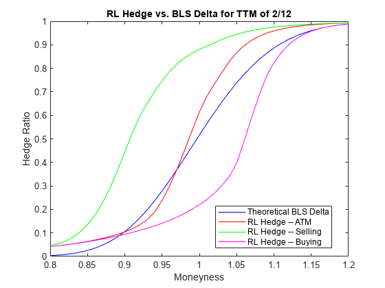
A plot of the hedge Ratio with respect to moneyness shows the differences between the BSM and RL approaches. As discussed in Cao [2], in the presence of transaction costs, the agent learns that "when delta hedging would require shares to be purchased, it tends to be optimal for a trader to be underhedged relative to delta. Similarly, when delta hedging would require shares to be sold, it tends to be optimal for a trader to be over-hedged relative to delta."
policy_RL_mR = @(mR,TTM,Pos) cell2mat(getAction(agent,[mR TTM Pos]'));

mRange = (.8:.01:1.2)';

figure
t_plot = 2/12;
plot(mRange,blsdelta(mRange,1,rfRate,t_plot,ExpVol),'b')
hold on
plot(mRange,arrayfun(@(mR) policy_RL_mR(mR,t_plot,blsdelta(mR,1,rfRate,t_plot,ExpVol)),mRange),'r')
plot(mRange,arrayfun(@(mR) policy_RL_mR(mR,t_plot,blsdelta(mR+.1,1,rfRate,t_plot,ExpVol)),mRange),'g')
plot(mRange,arrayfun(@(mR) policy_RL_mR(mR,t_plot,blsdelta(mR-.1,1,rfRate,t_plot,ExpVol)),mRange),'m')
legend('Theoretical BLS Delta','RL Hedge -- ATM','RL Hedge -- Selling','RL Hedge -- Buying', ...
    'location','best')
xlabel('Moneyness')
ylabel('Hedge Ratio')
title('RL Hedge vs. BLS Delta for TTM of 2/12')

References
[1] Buehler H., L. Gonon, J. Teichmann, and B. Wood. "Deep hedging." Quantitative Finance. Vol. 19, No. 8, 2019, pp. 1271–91.
[2] Cao J., J. Chen, J. Hull, and Z. Poulos. "Deep Hedging of Derivatives Using Reinforcement Learning." The Journal of Financial Data Science. Vol. 3, No. 1, 2021, pp. 10–27.
[3] Halperin I. "QLBS: Q-learner in the Black-Scholes (-Merton) Worlds." The Journal of Derivatives. Vol. 28, No. 1, 2020, pp. 99–122.
[4] Kolm P.N. and G. Ritter. "Dynamic Replication and Hedging: A Reinforcement Learning Approach." The Journal of Financial Data Science. Vol. 1, No. 1, 2019, pp. 159–71.
Local Functions
function [InitialObservation,LoggedSignals] = resetFcn(Moneyness,TimeToMaturity,InitPosition)
% Reset function to reset at the beginning of each episode.

LoggedSignals.State = [Moneyness TimeToMaturity InitPosition]';
InitialObservation  = LoggedSignals.State;

end

function [NextObs,Reward,IsDone,LoggedSignals] = stepFcn(Position_next,LoggedSignals,r,vol,dT,X,mu,c,kappa)
% Step function to evaluate at each step of the episode.

Moneyness_prev = LoggedSignals.State(1);
TTM_prev = LoggedSignals.State(2);
Position_prev = LoggedSignals.State(3);

S_prev = Moneyness_prev*X;

% GBM Motion
S_next = S_prev*((1 + mu*dT) + (randn* vol).*sqrt(dT));
TTM_next = max(0,TTM_prev - dT);

IsDone = TTM_next < eps;

stepReward = (S_next - S_prev)*Position_prev - abs(Position_next - Position_prev)*S_next*kappa - ...
    blsprice(S_next,X,r,TTM_next,vol) + blsprice(S_prev,X,r,TTM_prev,vol);

if IsDone
    stepReward = stepReward - Position_next*S_next*kappa;
end

Reward = stepReward - c*stepReward.^2;

LoggedSignals.State = [S_next/X;TTM_next;Position_next];
NextObs = LoggedSignals.State;

end

function perCosts = computeCosts(policy,nTrials,nSteps,SpotPrice,Strike,T,r,ExpVol,InitPos,dT,mu,kappa)
% Helper function to compute costs for any hedging approach.

rng(0)

simOBJ = gbm(mu,ExpVol,'StartState',SpotPrice);
[simPaths,simTimes] = simulate(simOBJ,nSteps,'nTrials',nTrials,'deltaTime',dT);
simPaths = squeeze(simPaths);

rew = zeros(nSteps,nTrials);

Position_prev = InitPos;
Position_next = policy(simPaths(1,:)/Strike,T*ones(1,nTrials),InitPos*ones(1,nTrials));
for timeidx=2:nSteps+1
    rew(timeidx-1,:) = (simPaths(timeidx,:) - simPaths(timeidx-1,:)).*Position_prev - ...
        abs(Position_next - Position_prev).*simPaths(timeidx,:)*kappa - ...
        blsprice(simPaths(timeidx,:),Strike,r,max(0,T - simTimes(timeidx)),ExpVol) + ...
        blsprice(simPaths(timeidx-1,:),Strike,r,T - simTimes(timeidx-1),ExpVol);

    if timeidx == nSteps+1
         rew(timeidx-1,:) =  rew(timeidx-1,:) - Position_next.*simPaths(timeidx,:,:)*kappa;
    else
        Position_prev = Position_next;
        Position_next = policy(simPaths(timeidx,:,:)/Strike,(T - simTimes(timeidx)).*ones(1,nTrials),Position_prev);
    end
end

perCosts = sum(rew);

end
See Also
blsprice | blsdelta | rlDDPGAgent (Reinforcement Learning Toolbox)