estimateCustomObjectivePortfolio

Estimate optimal portfolio for user-defined objective function for Portfolio object

Since R2022b

Syntax

[pwgt,pbuy,psell,exitflag] = estimateCustomObjectivePortfolio(obj,fun)

[pwgt,pbuy,psell,exitflag] = estimateCustomObjectivePortfolio(___,Name=Value)

Description

[pwgt,pbuy,psell,exitflag] = estimateCustomObjectivePortfolio(obj,fun) estimates optimal portfolio with a user-defined objective function for a Portfolio object. For details on using estimateCustomObjectivePortfolio, see Solver Guidelines for Custom Objective Problems Using Portfolio Objects.

[pwgt,pbuy,psell,exitflag] = estimateCustomObjectivePortfolio(___,Name=Value) adds optional name-value arguments.

Examples

Solve Continuous Problems Using Custom Objectives

This example shows how to use estimateCustomObjectivePortfolio to solve a portfolio problem with a custom objective. You define the constraints for portfolio problems using functions for the Portfolio object and then you specify the objective function as an input to estimateCustomObjectivePortfolio. The objective function must be continuous (and preferably smooth).

Create Portfolio Object

Find the portfolio that solves the problem:

$$\begin{array}{l}\underset{\mathit{x}}{\min }{\mathit{x}}^{\mathit{T}}\mathit{x}\\ \mathit{s}.\mathit{t}.\sum _{\mathit{i}}{\mathit{x}}_{\mathit{i}}=1\\ \mathit{x}\ge 0\end{array}$$

Create a Portfolio object and set the default constraints using setDefaultConstraints. In this case, the portfolio problem does not involve the mean or covariance of the assets returns. Therefore, you do not need to define the assets moments to create the Portfolio object. You need only to define the number of assets in the problem.

% Create a Portfolio object
p = Portfolio(NumAssets=6);
% Define the constraints of the portfolio methods
p = setDefaultConstraints(p); % Long-only, fully invested weights

Define Objective Function

Define a function handle for the objective function ${\mathit{x}}^{\mathit{T}}\mathit{x}$.

% Define the objective function
objFun = @(x) x'*x;

Solve Portfolio Problem

Use estimateCustomObjectivePortfolio to compute the solution to the problem.

% Solve portfolio problem
wMin = estimateCustomObjectivePortfolio(p,objFun)

wMin = 6×1

    0.1667
    0.1667
    0.1667
    0.1667
    0.1667
    0.1667

The estimateCustomObjectivePortfolio function automatically assumes that the objective sense is to minimize. You can change that default behavior by using the estimateCustomObjectivePortfolio name-value argument ObjectiveSense='maximize'.

Add Gross or Net Return Constraints for Problems with Custom Objectives

This example shows how to use estimateCustomObjectivePortfolio to solve a portfolio problem with a custom objective and a return constraint. You define the constraints for portfolio problems, other than the return constraint, using functions for the Portfolio object and then you specify the objective function as an input to estimateCustomObjectivePortfolio. The objective function must be continuous (and preferably smooth). To specify a return constraint, you use the TargetReturn name-value argument.

Create Portfolio Object

Find the portfolio that solves the problem:

$$\begin{array}{l}\underset{\mathit{x}}{\min }{\mathit{x}}^{\mathit{T}}\mathit{x}\\ \mathit{s}.\mathit{t}.\sum _{\mathit{i}}{\mathit{x}}_{\mathit{i}}=1\\ \mathit{x}\ge 0\end{array}$$

Create a Portfolio object and set the default constraints using setDefaultConstraints.

% Create a Portfolio object
load('SixStocks.mat')
p = Portfolio(AssetMean=AssetMean,AssetCovar=AssetCovar);
% Define the constraints of the portfolio methods
p = setDefaultConstraints(p); % Long-only, fully invested weights

Define Objective Function

Define a function handle for the objective function ${\mathit{x}}^{\mathit{T}}\mathit{x}$.

% Define the objective function
objFun = @(x) x'*x;

Add Return Constraints

When using the Portfolio object, you can use estimateFrontierByReturn to add a return constraint to the portfolio. However, when using the estimateCustomObjectivePortfolio function with a Portfolio object, you must add return constraints by using the TargetReturn name-value argument with a return target value.

The Portfolio object supports two types of return constraints: gross return and net return. The type of return constraint that is added to the portfolio problem is implicitly defined by whether you provide buy or sell costs to the Portfolio object using setCosts. If no buy or sell costs are present, the added return constraint is a gross return constraint. Otherwise, a net return constraint is added.

Gross Return Constraint

The gross portfolio return constraint for a portfolio is

$${\mathit{r}}_0+{\left(\mu -{\mathit{r}}_0\right)}^{\mathit{T}}\mathit{x}\ge {\mu }_0,$$

where ${\mathit{r}}_0$ is the risk-free rate (with 0 as default), $\mu$ is the mean of assets returns, and ${\mu }_0$ is the target return.

Since buy or sell costs are not needed to add a gross return constraint, the Portfolio object does not need to be modified before using estimateCustomObjectivePortfolio.

% Set a return target
ret0 = 0.03;
% Solve portfolio problem with a gross return constraint
wGross = estimateCustomObjectivePortfolio(p,objFun, ...
    TargetReturn=ret0)

wGross = 6×1

    0.1377
    0.1106
    0.1691
    0.1829
    0.1179
    0.2818

The return constraint is not added to the Portfolio object. In other words, the Portfolio properties are not modified by adding a gross return constraint in estimateCustomObjectivePortfolio.

Net Return Constraint

The net portfolio return constraint for a portfolio is

$${\mathit{r}}_0+{\left(\mu -{\mathit{r}}_0\right)}^{\mathit{T}}\mathit{x}-{\mathit{c}}_{\mathit{B}}^{\mathit{T}}\max \left\{0,\mathit{x}-{\mathit{x}}_0\right\}-{\mathit{c}}_{\mathit{S}}^{\mathit{T}}\max \left\{0,{\mathit{x}}_0-\mathit{x}\right\}\ge {\mu }_0,$$

where ${\mathit{r}}_0$ is the risk-free rate (with 0 as default), $\mu$ is the mean of assets returns, ${\mathit{c}}_{\mathit{B}}$ is the proportional buy cost, ${\mathit{c}}_{\mathit{S}}$ is the proportional sell cost, ${\mathit{x}}_0$ is the initial portfolio, and ${\mu }_0$ is the target return.

To add net return constraints to the portfolio problem, you must use setCosts with the Portfolio object. If the Portfolio object has either of these costs, estimateCustomObjectivePortfolio automatically assumes that any added return constraint is a net return constraint.

% Add buy and sell costs to the Portfolio object
buyCost = 0.002;
sellCost = 0.001;
initPort = zeros(p.NumAssets,1);
p = setCosts(p,buyCost,sellCost,initPort);
% Solve portfolio problem with a net return constraint
% wNet = estimateCustomObjectivePortfolio(p,objFun, ...
%    TargetReturn=ret0)

As with the gross return constraint, the net return constraint is not added to the Portfolio object properties, however the Portfolio object is modified by the addition of buy or sell costs. Adding buy or sell costs to the Portfolio object does not affect any constraints besides the return constraint, but these costs do affect the solution of maximum return problems because the solution is the maximum net return instead of the maximum gross return.

Solve Portfolio Problems with Custom Objectives and Cardinality Constraints

This example shows how to use estimateCustomObjectivePortfolio to solve a portfolio problem with a custom objective and cardinality constraints. You define the constraints for portfolio problems using functions for the Portfolio object and then you specify the objective function as an input to estimateCustomObjectivePortfolio. For problems with cardinality constraints or continuous bounds, the objective function must be continuous and convex.

Create Portfolio Object

Find a long-only, fully weighted portfolio with half the assets that minimizes the tracking error to the equally weighted portfolio. Furthermore, if an asset is present in the portfolio, at least 10% should be invested in that asset. The portfolio problem is as follows:

$$\begin{array}{l}\underset{\mathit{x}}{\min }{\left(\mathit{x}-{\mathit{x}}_0\right)}^{\mathit{T}}\Sigma \left(\mathit{x}-{\mathit{x}}_0\right)\\ \mathit{s}.\mathit{t}.\sum _{\mathit{i}}{\mathit{x}}_{\mathit{i}}=1,\\ \sum _{\mathit{i}}\mathit{\#}\left({\mathit{x}}_{\mathit{i}}\ne 0\right)=3,\\ {\mathit{x}}_{\mathit{i}}\ge 0.1\mathrm{or}{\mathit{x}}_{\mathit{i}}=0\end{array}$$

Create a Portfolio object and set the assets moments.

load('SixStocks.mat')
p = Portfolio(AssetMean=AssetMean,AssetCovar=AssetCovar);
nAssets = size(AssetMean,1);

Define the Portfolio constraints.

% Fully invested portfolio
p = setBudget(p,1,1);
% Cardinality constraint
p = setMinMaxNumAssets(p,3,3);
% Conditional bounds
p = setBounds(p,0.1,[],BoundType="conditional");

Define Objective Function

Define a function handle for the objective function.

% Define the objective function
EWP = 1/nAssets*ones(nAssets,1);
trackingError = @(x) (x-EWP)'*p.AssetCovar*(x-EWP);

Solve Portfolio Problem

Use estimateCustomObjectivePortfolio to compute the solution to the problem.

% Solve portfolio problem
wMinTE = estimateCustomObjectivePortfolio(p,trackingError)

wMinTE = 6×1

    0.1795
    0.3507
         0
    0.4698
         0
         0

Using ObjectiveBound and InitialPoint with Custom Objective Portfolios

This example shows how to use the name-value arguments ObjectiveBound and InitialPoint with estimateCustomObjectivePortfolio.

Load the returns data in CAPMuniverse.mat. Then, create a standard mean-variance Portfolio object with default constraints, which is a long-only portfolio whose weights sum to 1. For this example, you can define the feasible region of weights $\mathit{X}$ as

$$\mathit{X}=\left\{\mathit{x}|\sum _{\mathit{i}=1}^{\mathit{n}}{\mathit{x}}_{\mathit{i}}=1,{\mathit{x}}_{\mathit{i}}\ge 0\right\}.$$

% Load data
load CAPMuniverse

% Create a mean-variance Portfolio object with default constraints
p = Portfolio(AssetList=Assets(1:12));
p = estimateAssetMoments(p,Data(:,1:12));
p = setDefaultConstraints(p);

% Add conditional bounds
pInt = setBounds(p,0.1,[],BoundType='cond');

Using ObjectiveBound

Use the ObjectiveBound name-value argument to provide an initial bound for the objective function. Providing an initial bound saves computation time because the solver does not have to solve an initial NLP relaxation to obtain the initial bound. Set up the MINLP solver, then test its performance when you do not provide an initial bound.

% Minimize tracking error without a lower bound
wTE = 1/p.NumAssets*ones(p.NumAssets,1);
trackingError = @(w) (w-wTE)'*p.AssetCovar*(w-wTE);
pInt2 = setSolverMINLP(pInt,'OuterApproximation',...
    ExtendedFormulation=true);
s = tic;
wTE_NoBound = estimateCustomObjectivePortfolio(pInt2,trackingError);
timeTE_NoBound = toc(s)

timeTE_NoBound = 7.5143

Since the lowest value that can be achieved by the tracking error is 0, you can use that as the lower bound with the ObjectiveBound name-value argument. Test the solver's performance when you do provide this lower bound. The solver is much faster when you provide one.

% Minimize tracking error with a lower bound
s = tic;
wTE_WithBound = estimateCustomObjectivePortfolio(pInt2,trackingError,ObjectiveBound=0);
timeTE_WithBound = toc(s)

timeTE_WithBound = 1.5837

Because you are minimizing the objective function, the bound that you provide to estimateCustomObjectivePortfolio must be a lower bound.

If you want to maximize the objective, then when you set ObjectiveSense to 'maximize', the ObjectiveBound is the upper bound of the objective function. Maximize the Sharpe ratio using ObjectiveBound.

% Maximize Sharpe ratio with upper bound
sharpeRatio = @(x) (p.AssetMean'*x)/sqrt(x'*p.AssetCovar*x);
wSR = estimateCustomObjectivePortfolio(pInt,sharpeRatio,...
    ObjectiveSense='maximize',ObjectiveBound=1);

Note that the ObjectiveBound name-value argument is ignored in continuous problems.

Using InitialPoint

Use the InitialPoint name-value argument to provide an initial point to the Portfolio solvers at the beginning of the iterations. You can use this name-value argument in continuous problems with nonconvex objectives to search the feasible region to find different local minima.

Set up a risk parity portfolio with constraints, group the constraints, then estimate the portfolio without and with specifying an initial point. Compare the risk parities of these portfolios.

% Risk parity portfolio with constraints
sigma = [5;5;7;10;15;15;15;18]/100;
rho = [ 1    0.8  0.6 -0.2 -0.1 -0.2 -0.2 -0.2;
        0.8  1    0.4 -0.2 -0.2 -0.1 -0.2 -0.2;
        0.6  0.4  1    0.5  0.3  0.2  0.2  0.3;
       -0.2 -0.2  0.5  1    0.6  0.6  0.5  0.6;
       -0.1 -0.2  0.3  0.6  1    0.9  0.7  0.7;
       -0.2 -0.1  0.2  0.6  0.9  1    0.6  0.7;
       -0.2 -0.2  0.2  0.5  0.7  0.6  1    0.7;
       -0.2 -0.2  0.3  0.6  0.7  0.7  0.7  1];
covariance = corr2cov(sigma,rho);
riskParity = @(x) sum((x.*(covariance*x)/(x'*covariance*x)-1).^2);

% Group the contraints
p = Portfolio(NumAssets=8);
p = setDefaultConstraints(p);
G = [0 0 0 0 1 1 1 1];
p = setGroups(p,G,0.3,[]);

% Solve the problem
w = estimateCustomObjectivePortfolio(p,riskParity);
riskParity(w)

ans = 6.1365

% Use the InitialPoint name-value argument
x0 = [0.7; zeros(3,1); 0.3; zeros(3,1)];
w2 = estimateCustomObjectivePortfolio(p,riskParity,InitialPoint=x0);
riskParity(w2)

ans = 6.1667

The objective function is different for different initial portfolios, because the objective function used to compute the risk parity portfolios is nonconvex.

Using different initial points in mixed-integer problems should not return different values of the objective function because the objective function should always be convex. That is, there is only one value for the minimum of the objective function.

Add Tracking Error Constraints to a Custom Objective Problem

This example shows how to use estimateCustomObjectivePortfolio to compare the weight assignment of the minimum risk portfolio with a constrained equally weighted portfolio. The weights can be either zero or greater than 15% and must sum to 1. You define the constraints for portfolio problems using functions for the Portfolio object and then you specify the objective function as an input to estimateCustomObjectivePortfolio. The objective function must be continuous (and preferably smooth).

Create Portfolio Object

Create a Portfolio object and set the bounds and budget using setBounds and setBudget.

% Define initial data
m = [ 0.05; 0.1; 0.12; 0.18 ];
C = [ 0.0064 0.00408 0.00192 0; 
    0.00408 0.0289 0.0204 0.0119;
    0.00192 0.0204 0.0576 0.0336;
    0 0.0119 0.0336 0.1225 ];

% Create Portfolio object
p = Portfolio(AssetMean=m,AssetCovar=C);

% Weight bounds
p1 = setBounds(p,0.15,1,BoundType='conditional');
% Weights must sum to one
p1 = setBudget(p1,1,1);

Add a tracking error constraint using setTrackingError to bound deviations from the max Sharpe ratio portfolio to 3%.

% Compute max Sharpe ratio portfolio
wSR = estimateMaxSharpeRatio(p1,Method='iterative');

% Set tracking error constraint
p1 = setTrackingError(p1,0.03,wSR);

Solve and compare the minimum risk portfolio and the constrained equally weighted portfolio.

% Compute max return portfolio
wMin = estimateFrontierLimits(p1,'min');

% Compute equally weighted portfolio by minimizing the
% Herfindahl-Hirshman index
HH = @(w) w'*w;
wHH = estimateCustomObjectivePortfolio(p1,HH);

Use a bar plot to observe the difference between the portfolios.

figure
bar([wMin wHH wSR])
legend('Minimum Risk','Equally Weighted','Max Sharpe')

Notice that the weights of the minimum risk portfolio are closer to the weights of the max Sharpe ratio than the weights of the constrained equally weighted portfolio (EWP). This happens because the priority of the constrained EWP is to make the weights as even as possible while still satisfying the constraints. Thus, the weights of the EWP are closer to each other than the rest of the portfolios.

Add Risk Constraint to a Custom Objective Problem

This example shows how to use estimateCustomObjectivePortfolio to define a risk-constrained long-only, fully-invested portfolio and then compare the maximum return portfolio against a minimum tracking error portfolio, where the tracking portfolio is the equally-weighted portfolio. You define the constraints for portfolio problems using functions for the Portfolio object and then you specify the objective function as an input to estimateCustomObjectivePortfolio. The objective function must be continuous (and preferably smooth).

Create Portfolio Object

Create a Portfolio object using the default constraints and then define the targetRisk.

% Define initial data
m = [ 0.05; 0.1; 0.12; 0.18 ];
C = [ 0.0064 0.00408 0.00192 0; 
    0.00408 0.0289 0.0204 0.0119;
    0.00192 0.0204 0.0576 0.0336;
    0 0.0119 0.0336 0.1225 ];

% Create Portfolio object
p = Portfolio(AssetMean=m,AssetCovar=C);

% Set long-only, fully-invested constraints
p2 = setDefaultConstraints(p);

% Define maximum risk of the portfolio
targetRisk = 0.1;

To compute the maximum return portfolio subject to a risk constraint, use estimateFrontierByRisk.

% Compute the max return risk constrained portfolio
wMax = estimateFrontierByRisk(p2,targetRisk);

Compute the minimum tracking error portfolio subject to a risk constraint using estimateCustomObjectivePortfolio, where the tracking portfolio is the equally weighted portfolio.

% Compute the min tracking error portfolio with a risk constraint
x0 = 1/4*ones(4,1);
TE = @(w) (w-x0)'*p2.AssetCovar*(w-x0);
wTE = estimateCustomObjectivePortfolio(p2,TE,...
    TargetVolatility=targetRisk);

Use a bar plot to observe the difference between the portfolios.

figure
bar([wMax wTE])
legend('Max Return','Min TE')

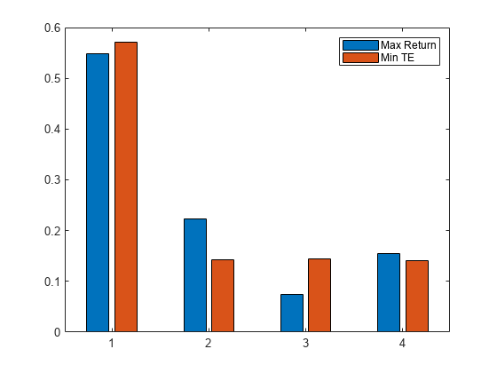
Notice that the weights of the minimum tracking portfolio tries to keep the weights of the assets more evenly weighted. However, in order to satisfy the risk constraint, the minimum tracking error portfolio still allocates a larger weight to the less risky asset.

Input Arguments

obj — Object for portfolio optimization

Portfolio object

Object for portfolio optimization, specified using a Portfolio object. When using a Portfolio object in the custom objective workflow, you do not need to specify the mean and covariance. However, the custom objective workflow requires that you specify either the mean, the covariance, or the number of assets.

Note

If no initial portfolio is specified in obj.InitPort, the initial portfolio is assumed to be 0 so that pbuy = max(0, pwgt) and psell = max(0, -pwgt). If no tracking portfolio is specified in obj.TrackingPort, the tracking portfolio is assumed to be 0.

Data Types: object

fun — Function handle that defines objective function

function handle

Function handle that defines the objective function, specified using a function handle in terms of the portfolio weights.

Note

The objective function must be continuous and defined using only the portfolio weights as variables. If the portfolio problem has cardinality constraints and/or conditional bounds using setMinMaxNumAssets or setBounds, the objective function must also be convex. For more information, see Role of Convexity in Portfolio Problems.

Data Types: function_handle

Name-Value Arguments

Specify optional pairs of arguments as Name1=Value1,...,NameN=ValueN, where Name is the argument name and Value is the corresponding value. Name-value arguments must appear after other arguments, but the order of the pairs does not matter.

Example: pwgt = estimateCustomObjectivePortfolio(p,fun,ObjectiveSense="maximize",TargetReturn=0.05)

ObjectiveSense — Sense of optimization

"minimize" (default) | string with value "mimimize" or "maximize" | character vector with value 'mimimize' or 'maximize'

Sense of the optimization, specified as ObjectiveSense and a string or character vector with one of the following values:

• "minimize" — The solution minimizes the objective function.

• "maximize" — The solution maximizes the objective function.

Data Types: string | char

TargetReturn — Target value for portfolio return

[] (default) | scalar

Target value for portfolio return, specified as TargetReturn and a scalar numeric value. For an example, see Add Gross or Net Return Constraints for Problems with Custom Objectives.

Data Types: double

TargetVolatility — Target value for portfolio standard deviation

[] (default) | nonnegative scalar

Since R2024a

Target value for portfolio standard deviation, specified as TargetVolatility and a nonnegative scalar numeric value. For an example, see Add Risk Constraint to a Custom Objective Problem.

Data Types: double

ObjectiveBound — User-supplied objective function bound

[] (default) | numeric

Since R2023b

User-supplied objective function bound, specified as ObjectiveBound and a numeric value. ObjectiveBound is useful to speed up solvers.

Note

If ObjectiveSense is 'minimize', then ObjectiveBound should be a lower bound of the objective function. If ObjectiveSense is 'maximize', then ObjectiveBound should be an upper bound of the objective function. If ObjectiveBound is not specified, a numerical lower bound is computed.

Data Types: double

InitialPoint — Weights allocation to initialize solver

[] (default) | vector

Since R2023b

Weights allocation to initialize solver, specified as InitialPoint and a NumAssets-by-1 vector. InitialPoint is useful for continuous portfolio problems that may have many local minima. By specifying a starting point, you can make the algorithm search different local minima.

Note

If InitialPoint is not specified, it is set to the long-only, fully-invested, equally-weighted portfolio.

Data Types: double

Output Arguments

pwgt — Optimal weight allocation of portfolio problem

vector

Optimal weight allocation of the portfolio problem, returned as a NumAssets-by-1 vector.

pbuy — Purchases relative to initial portfolio to achieve optimal weight allocation of portfolio problem

vector

Purchases relative to initial portfolio to achieve the optimal weight allocation of the portfolio problem, returned as a NumAssets-by-1 vector.

psell — Sales relative to initial portfolio to achieve optimal weight allocation of the portfolio problem

vector

Sales relative to initial portfolio to achieve the optimal weight allocation of the portfolio problem, returned as a NumAssets vector.

exitflag — Reason solver stopped

enumeration variable | integer

Reason the solver stopped, returned as an enumeration variable or integer. There are two types of exitflag output. If the problem is continuous, the exitflag output is an enumeration variable. If the problem is mixed-integer, then the exitflag output is an integer.

References

[1] Cornuejols, G. and Reha Tütüncü. Optimization Methods in Finance. Cambridge University Press, 2007.

Version History

Introduced in R2022b

R2024a: Support tracking error constraints

estimateCustomObjectivePortfolio supports tracking error constraints when using setTrackingError with the Portfolio object. For an example, see Add Tracking Error Constraints to a Custom Objective Problem.

R2024a: Added Name-Value Arguments for TargetVolatility for risk constraints

estimateCustomObjectivePortfolio added a name-value argument for TargetVolatility for risk constraints. For an example, see Add Risk Constraint to a Custom Objective Problem.

R2023b: Added Name-Value Arguments for ObjectiveBound and InitialPoint

estimateCustomObjectivePortfolio added name-value arguments for ObjectiveBound and InitialPoint.