Implement HDL Optimized SVD in Feedforward Fashion Without Backpressure
This example shows how to implement a hardware-efficient singular value decomposition (SVD) using the Square Jacobi SVD HDL Optimized block in a feedforward fashion without backpressure.
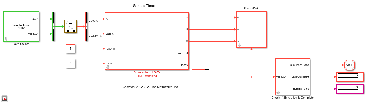
The Square Jacobi SVD HDL Optimized block uses the AMBA AXI handshake protocol for both input and output. To use the block without backpressure control, feed a constant Boolean 'true' to the readyIn port, then configure the upstream input rate according to the block latency specified in Square Jacobi SVD HDL Optimized.
This model uses a Rate Transition block between the data source and the Square Jacobi SVD HDL Optimized block to emulate an upstream block with a lower sample rate. The sample time of the Square Jacobi SVD HDL Optimized block is normalized to 1, and the sample time of data source is the block latency + 1.
Define Simulation Parameters
Specify the dimension of the sample matrices, the number of input sample matrices, and the number of iterations of the Jacobi algorithm.
n = 8;
numSamples = 3;
nIterations = 6;
Generate Input A Matrices
Use the specified simulation parameters to generate the input A matrices.
rng('default');
A = randn(n,n,numSamples);
The Square Jacobi SVD HDL Optimized block supports both real and complex inputs. Set the complexity of the input in the block mask accordingly.
% A = complex(randn(n,n,numSamples),randn(n,n,numSamples));
Select Fixed-Point Data Types
Define the desired word length.
wordLength = 32;
Use the upper bound on the singular values to define fixed-point types that will never overflow. First, use the fixed.singularValueUpperBound function to determine the upper bound on the singular values.
svdUpperBound = fixed.singularValueUpperBound(n,n,max(abs(A(:))));
Define the integer length based on the value of the upper bound, with one additional bit for the sign, another additional bit for intermediate CORDIC growth, and one more bit for intermediate growth to compute the Jacobi rotations.
additionalBitGrowth = 3;
integerLength = ceil(log2(svdUpperBound)) + additionalBitGrowth;
Compute the fraction length based on the integer length and the desired word length.
fractionLength = wordLength - integerLength;
Define the signed fixed-point data type to be 'Fixed' or 'ScaledDouble'. You can also define the type to be 'double' or 'single'.
dataType = 'Fixed';
T.A = fi([],1,wordLength,fractionLength,'DataType',dataType);
disp(T.A)
[]

          DataTypeMode: Fixed-point: binary point scaling
            Signedness: Signed
            WordLength: 32
        FractionLength: 24
Cast the matrix A to the signed fixed-point type.
A = cast(A,'like',T.A);
Set Input Rate
The latency of the Square Jacobi SVD HDL Optimized block depends on the size n, complexity, and word length wl of the input matrix A, and the number of iterations nIterations of the two-sided Jacobi algorithm.
If signal complexity is real, the block delay is
(wl*2+31)*(n-1+rem(n,2))*nIterations+2+nextpow2(n)*(nextpow2(n)+1)/2+3.If signal complexity is complex, the block delay is
(wl*6+48)*(n-1+rem(n,2))*nIterations+2+nextpow2(n)*(nextpow2(n)+1)/2+3.If
Ais double precision, thenwlis53.if
Ais single precision, thenwlis24.
The Square Jacobi SVD HDL Optimized block will be ready in the next clock after a successful solution output. Therefore, the input rate transition ratio should be at least 1 + block latency.
For real input, compute the rate transition ratio.
rateTransitionRatio = 1+(wordLength*2+31)*(n-1+rem(n,2))*nIterations+2+nextpow2(n)*(nextpow2(n)+1)/2+3;
For complex input, compute the rate transition ratio.
% rateTransitionRatio = 1+(wordLength*6+48)*(n-1+rem(n,2))*nIterations+2+nextpow2(n)*(nextpow2(n)+1)/2+3;
Configure Model Workspace and Run Simulation
model = 'SquareJacobiSVDFeedforwardModel';
open_system(model);
fixed.example.setModelWorkspace(model,'A',A,'n',n,...
    'nIterations',nIterations,'numSamples',numSamples,...
    'rateTransitionRatio',rateTransitionRatio);
out = sim(model);
Verify Output Solutions
Verify the output solutions. In these steps, "identical" means within roundoff error.
Verify that
U*diag(s)*V'is identical toA.relErrUSVrepresents the relative error betweenU*diag(s)*V'andA.Verify that the singular values
sare identical to the floating point SVD solution.relativeErrorSrepresents the relative error betweensand the singular values calculated by MATLAB®svdfunction.Verify that
UandVare unitary matrices.relativeErrorUUrepresents the relative error betweenU'*Uand the identity matrix.relativeErrorVVrepresents the relative error betweenV'*Vand the identity matrix.
for i = 1:numSamples
    disp(['Sample #',num2str(i),':']);
    a = A(:,:,i);
    U = out.U(:,:,i);
    V = out.V(:,:,i);
    s = out.s(:,:,i);

    % Verify U*diag(s)*V'
    if norm(double(a)) > 1
        relativeErrorUSV = norm(double(U*diag(s)*V')-double(a))/norm(double(a));
    else
        relativeErrorUSV = norm(double(U*diag(s)*V')-double(a));
    end
    relativeErrorUSV %#ok

    % Verify s
    s_expected = svd(double(a));
    normS = norm(s_expected);
    relativeErrorS = norm(double(s) - s_expected);
    if normS > 1
        relativeErrorS = relativeErrorS/normS;
    end
    relativeErrorS %#ok

    % Verify U'*U
    U = double(U);
    UU = U'*U;
    relativeErrorUU = norm(UU - eye(size(UU))) %#ok

    % Verify V'*V
    V = double(V);
    VV = V'*V;
    relativeErrorVV = norm(VV - eye(size(VV))) %#ok

    disp('---------------');
end
Sample #1:

relativeErrorUSV =

   3.3400e-06


relativeErrorS =

   9.5255e-07


relativeErrorUU =

   2.3165e-07


relativeErrorVV =

   3.2086e-07

---------------
Sample #2:

relativeErrorUSV =

   4.2501e-06


relativeErrorS =

   1.1657e-06


relativeErrorUU =

   2.6221e-07


relativeErrorVV =

   3.2105e-07

---------------
Sample #3:

relativeErrorUSV =

   4.0549e-06


relativeErrorS =

   1.3268e-06


relativeErrorUU =

   3.4778e-07


relativeErrorVV =

   2.3183e-07

---------------