Set Data Types Using Min/Max Instrumentation
In this example, you set fixed-point data types by instrumenting MATLAB® code for min/max logging then use the tools to propose data types. You use the buildInstrumentedMex function to build the MEX function with instrumentation enabled, then use the showInstrumentationResults to show instrumentation results and the clearInstrumentationResults function to clear instrumentation results.
Define the Unit Under Test
The function that you convert to fixed-point in this example is a second-order direct-form 2 transposed filter. You can substitute your own function in place of this one to reproduce these steps in your own work.
function [y,z] = fi_2nd_order_df2t_filter(b,a,x,y,z)
    for i=1:length(x)
        y(i) = b(1)*x(i) + z(1);
        z(1) = b(2)*x(i) + z(2) - a(2) * y(i);
        z(2) = b(3)*x(i)        - a(3) * y(i);
    end
end
For a MATLAB function to be instrumented, it must be suitable for code generation. For information on code generation, see the buildInstrumentedMex reference page. A MATLAB Coder™ license is not required to use the buildInstrumentedMex function.
In the function fi_2nd_order_df2t_filter, the variables y and z are used as both inputs and outputs. This is an important pattern because:
You can set the data type of
yandzoutside the function, thus allowing you to re-use the function for both fixed-point and floating-point types.The generated C code will create
yandzas references in the function argument list.
Use Design Requirements to Determine Data Types
In this example, the requirements of the design determine the data type of input x. These requirements are signed, 16-bit, and fractional.
clearvars
N = 256;
x = fi(zeros(N,1),1,16,15);
The requirements of the design also determine the fixed-point math for a DSP target with a 40-bit accumulator. This example uses floor rounding and wrap on overflow to produce efficient generated code.
F = fimath('RoundingMethod','Floor',...
           'OverflowAction','Wrap',...
           'ProductMode','KeepLSB',...
           'ProductWordLength',40,...
           'SumMode','KeepLSB',...
           'SumWordLength',40);
The following coefficients correspond to a second-order lowpass filter created by
[num,den] = butter(2,0.125)
The values of the coefficients influence the range of the values that will be assigned to the filter output and states.
num = [0.0299545822080925  0.0599091644161849  0.0299545822080925];
den = [1                  -1.4542435862515900  0.5740619150839550];
The data type of the coefficients, determined by the requirements of the design, are specified as 16-bit word length and scaled to best-precision. To create fi objects from constant coefficients:
1. Cast the coefficients to fi objects using the default round-to-nearest and saturate on overflow settings, which gives the coefficients better accuracy.
b = fi(num,1,16);
a = fi(den,1,16);
2. Attach fimath with floor rounding and wrap on overflow settings to control arithmetic, which leads to more efficient C code.
b = setfimath(b,F);
a = setfimath(a,F);
Use Values of the Coefficients and Inputs to Determine Data Types
The values of the coefficients and values of the inputs determine the data types of output y and state vector z. Create them with a scaled double datatype so their values will attain full range and you can identify potential overflows and propose data types.
yisd = fi(zeros(N,1),1,16,15,'DataType','ScaledDouble','fimath',F);
zisd = fi(zeros(2,1),1,16,15,'DataType','ScaledDouble','fimath',F);
Instrument the MATLAB Function as a Scaled-Double MEX Function
To instrument the MATLAB code, you create a MEX function from the MATLAB function using the buildInstrumentedMex function. The inputs to buildInstrumentedMex are the same as the inputs to fiaccel, but buildInstrumentedMex has no fi-object restrictions. The output of buildInstrumentedMex is a MEX function with instrumentation inserted. When the MEX function is run, the simulated minimum and maximum values are recorded for all named variables and intermediate values.
Use the '-o' option to name the MEX function that is generated. If you do not use the '-o' option, then the MEX function is the name of the MATLAB function with '_mex' appended. You can also name the MEX function the same as the MATLAB function, but you need to remember that MEX functions take precedence over MATLAB functions and so changes to the MATLAB function will not run until either the MEX function is re-generated, or the MEX function is deleted and cleared.
Hard-code the filter coefficients into the implementation of this filter by passing them as constants to the buildInstrumentedMex function.
Use the '-histogram' option to compute the log2 histogram for all named, intermediate, and expression values. These histograms appear in the code generation report table.
buildInstrumentedMex fi_2nd_order_df2t_filter ...
    -o filter_scaled_double ...
    -args {coder.Constant(b),coder.Constant(a),x,yisd,zisd} ...
    -histogram
Test Bench with Chirp Input
The test bench for this system is set up to run chirp and step signals. In general, test benches for systems should cover a wide range of input signals.
The first test bench uses a chirp input. A chirp signal is a good representative input because it covers a wide range of frequencies.
t = linspace(0,1,N);       % Time vector from 0 to 1 second
f1 = N/2;                  % Target frequency of chirp set to Nyquist
xchirp = sin(pi*f1*t.^2);  % Linear chirp from 0 to Fs/2 Hz in 1 second
x(:) = xchirp;             % Cast the chirp to fixed-point
Run the Instrumented MEX Function to Record Min/Max Values
The instrumented MEX function must be run to record minimum and maximum values for that simulation run. Subsequent runs accumulate the instrumentation results until they are cleared with clearInstrumentationResults.
Note that the numerator and denominator coefficients were compiled as constants so they are not provided as input to the generated MEX function.
ychirp = filter_scaled_double(b,a,x,yisd,zisd);
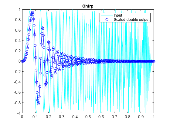
The plot of the filtered chirp signal shows the lowpass behavior of the filter with these particular coefficients. Low frequencies are passed through and higher frequencies are attenuated.
plot(t,x,'c',t,ychirp,'bo-')
title('Chirp')
legend('Input','Scaled-double output')
Show Instrumentation Results with Proposed Fraction Lengths for Chirp
The showInstrumentationResults function displays the code generation report with instrumented values. The input to the showInstrumentationResults function is the name of the instrumented MEX function for which you want to show results.
Potential overflows are only displayed for fi objects with Scaled Double data type.
This particular design is for a DSP where the word lengths are fixed, so use the -proposeFL flag to propose fraction lengths.
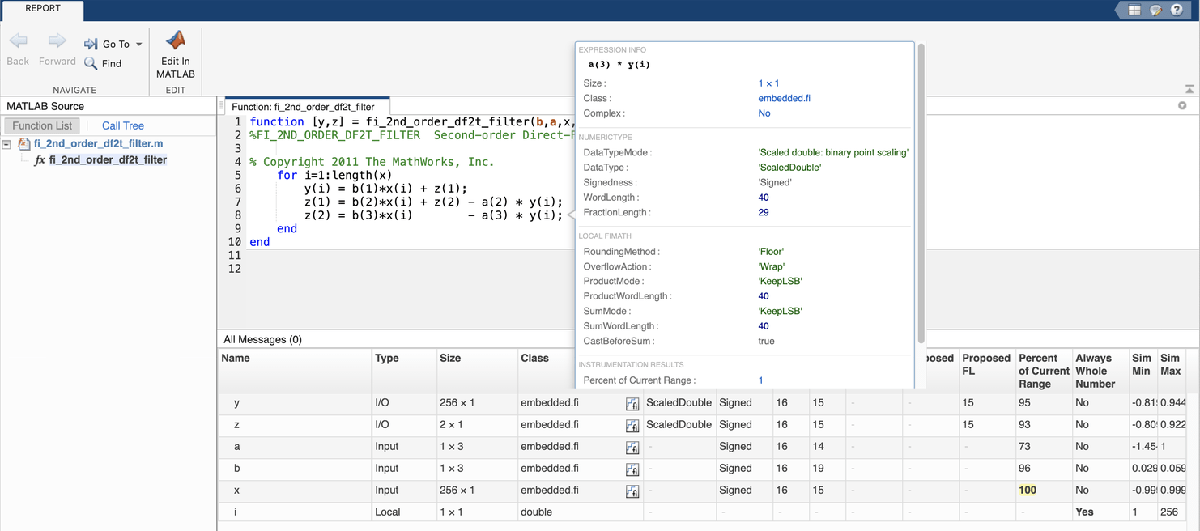
showInstrumentationResults filter_scaled_double -proposeFL
Hover over expressions or variables in the instrumented code generation report to see the simulation minimum and maximum values. In this design, the inputs fall between -1 and +1, and the values of all variables and intermediate results also fall between -1 and +1. This suggests that the data types can all be fractional (fraction length one bit less than the word length). However, this will not always be true for this function for other kinds of inputs and it is important to test many types of inputs before setting final fixed-point data types.
To view the histogram for a variable, click the histogram icon in the Variables tab.
Test Bench with Step Input
The next test bench is run with a step input. A step input is a good representative input because it is often used to characterize the behavior of a system.
xstep = [ones(N/2,1);-ones(N/2,1)];
x(:) = xstep;
Run the Instrumented MEX Function with Step Input
The instrumentation results are accumulated until they are cleared with clearInstrumentationResults.
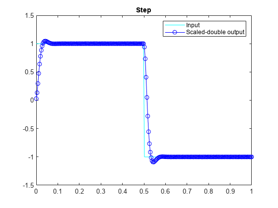
ystep = filter_scaled_double(b,a,x,yisd,zisd);

plot(t,x,'c',t,ystep,'bo-')
title('Step')
legend('Input','Scaled-double output')
Show Accumulated Instrumentation Results
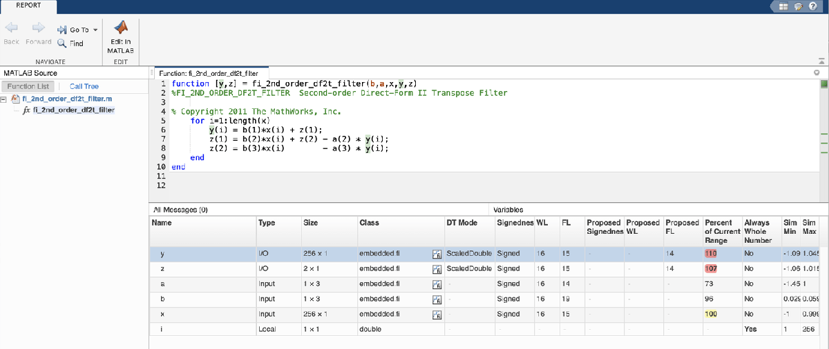
Even though the inputs for step and chirp inputs are both full range as indicated by x at 100 percent current range in the instrumented code generation report, the step input causes overflow while the chirp input did not. This is an illustration of the necessity to have many different inputs for your test bench. For the purposes of this example, only two inputs were used, but real test benches should be more thorough.
showInstrumentationResults filter_scaled_double -proposeFL
Apply Proposed Fixed-Point Properties
To prevent overflow, set proposed fixed-point properties based on the proposed fraction lengths of 14-bits for y and z from the instrumented code generation report.
At this point in the workflow, you use true fixed-point types (as opposed to the scaled double types that were used in the earlier step of determining data types).
yi = fi(zeros(N,1),1,16,14,'fimath',F);
zi = fi(zeros(2,1),1,16,14,'fimath',F);
Instrument the MATLAB Function as a Fixed-Point MEX Function
Create an instrumented fixed-point MEX function by using fixed-point inputs and the buildInstrumentedMex function.
buildInstrumentedMex fi_2nd_order_df2t_filter ...
    -o filter_fixed_point ...
    -args {coder.Constant(b),coder.Constant(a),x,yi,zi}
Validate the Fixed-Point Algorithm
After converting to fixed-point, run the test bench again with fixed-point inputs to validate the design.
Validate with Chirp Input
Run the fixed-point algorithm with a chirp input to validate the design.
x(:) = xchirp;
[y,z] = filter_fixed_point(b,a,x,yi,zi);
[ysd,zsd] = filter_scaled_double(b,a,x,yisd,zisd);
err = double(y) - double(ysd);
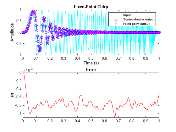
Compare the fixed-point outputs to the scaled-double outputs to verify that they meet your design criteria.
subplot(211);
plot(t,x,'c',t,ysd,'bo-',t,y,'mx')
xlabel('Time (s)');
ylabel('Amplitude')
legend('Input','Scaled-double output','Fixed-point output');
title('Fixed-Point Chirp')
subplot(212);
plot(t,err,'r');title('Error');xlabel('t'); ylabel('err');
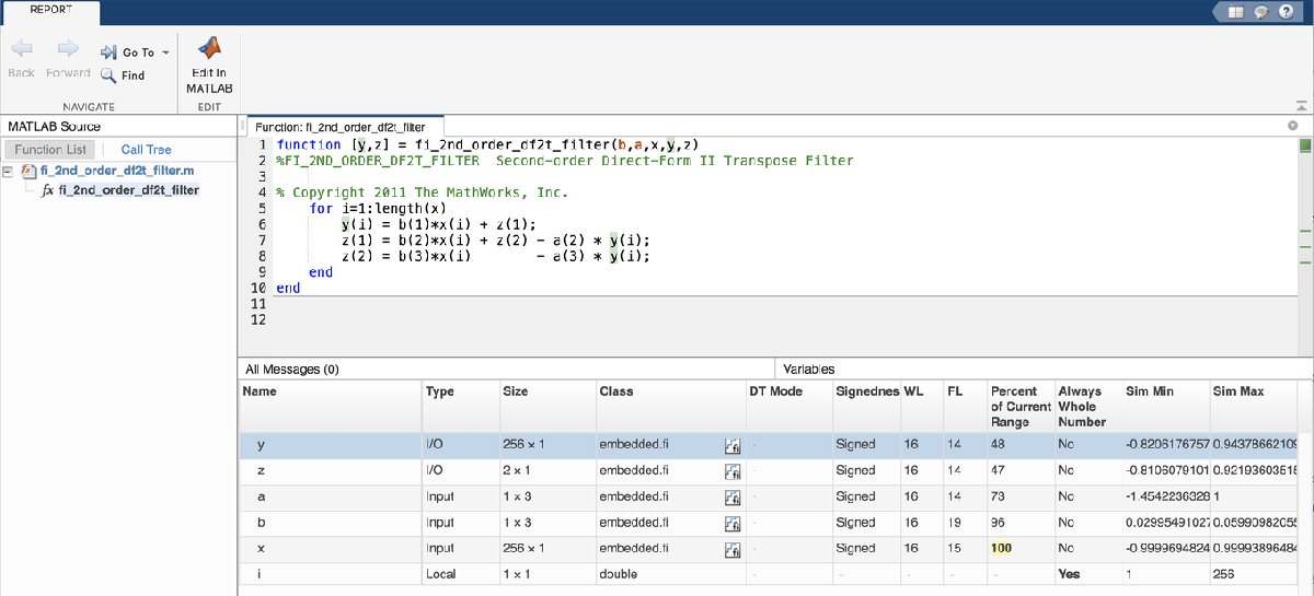
Inspect the variables and intermediate results to ensure that the min/max values are within range.
showInstrumentationResults filter_fixed_point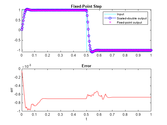
Validate with Step Inputs
Run the fixed-point algorithm with a step input to validate the design.
Run the following code to clear the previous instrumentation results to see only the effects of running the step input.
clearInstrumentationResults filter_fixed_pointRun the step input through the fixed-point filter and compare with the output of the scaled double filter.
x(:) = xstep;
[y,z] = filter_fixed_point(b,a,x,yi,zi);
[ysd,zsd] = filter_scaled_double(b,a,x,yisd,zisd);
err = double(y) - double(ysd);
Plot the fixed-point outputs against the scaled-double outputs to verify that they meet your design criteria.
subplot(211);
plot(t,x,'c',t,ysd,'bo-',t,y,'mx')
title('Fixed-Point Step');
legend('Input','Scaled-double output','Fixed-point output')
subplot(212);
plot(t,err,'r');title('Error');xlabel('t'); ylabel('err');
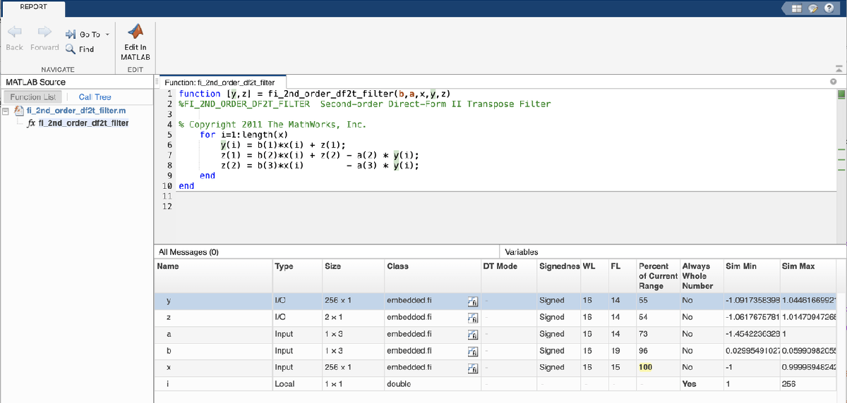
Inspect the variables and intermediate results to ensure that the min/max values are within range.
showInstrumentationResults filter_fixed_point
Suppress Code Analyzer warnings.
%#ok<*ASGLU>