Main Content

estimateStates

Batch fusion and smoothing of sensor data

Since R2022a

Description

example

estimates = estimateStates(filter,sensorData,measurementNoise) returns the state estimates based on the motion model used in the filter, the sensor data, and the measurement noise. The function predicts the filter state estimates forward in time based on the row times in sensorData and fuses data from each column of the table one by one.

example

[estimates,smoothEstimates] = estimateStates(___) additionally returns the smoothed state estimates by using the Rauch-Tung-Striebel (RTS) nonlinear Kalman smoother. For algorithm details, see Algorithms and [1].

Tip

Smoothing usually requires considerably more memory and computation time. Use this syntax only when you need the smoothed estimated states.

Examples

collapse all

Load measurement data from an accelerometer and a gyroscope.

load("accelGyroINSEKFData.mat");

Create an insEKF filter object. Specify the orientation part of the state in the filter using the initial orientation from the measurement data. Specify the diagonal elements of the state estimate error covariance matrix corresponding to the orientation state as 0.01.

filt = insEKF;
stateparts(filt,"Orientation",compact(initOrient));
statecovparts(filt,"Orientation",1e-2);

Specify the measurement noise and the additive process noise. You can obtain these values by using the tune object function of the filter object.

measureNoise = struct("AccelerometerNoise", 0.1739, ...
    "GyroscopeNoise", 1.1129);
processNoise = diag([ ...
    2.8586 1.3718 0.8956 3.2148 4.3574 2.5411 3.2148 0.5465 0.2811 ...
    1.7149 0.1739 0.7752 0.1739]);
filt.AdditiveProcessNoise = processNoise;

Batch-estimate the states using the estimateStates object function. Also, obtain the estimates after smoothing.

[estimates,smoothEstimates] = estimateStates(filt,sensorData,measureNoise);

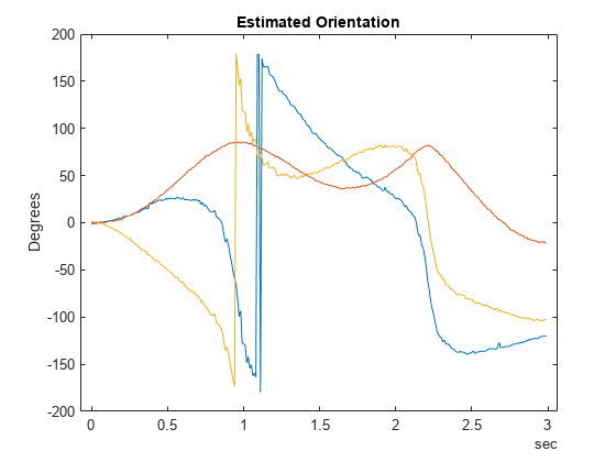
Visualize the estimated orientation in Euler angles.

figure
t = estimates.Properties.RowTimes;
plot(t,eulerd(estimates.Orientation,"ZYX","frame"));
title("Estimated Orientation");
ylabel("Degrees")

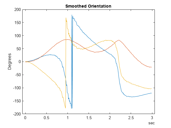
Visualize the estimated orientation after smoothing in Euler angles.

figure
plot(t,eulerd(smoothEstimates.Orientation,"ZYX","frame"));
title("Smoothed Orientation");
ylabel("Degrees")

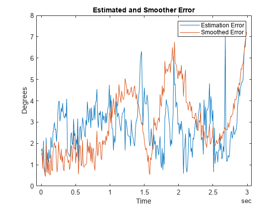
Visualize the estimate error, in quaternion distance, using the dist object function of the quaternion object.

trueOrient = groundTruth.Orientation;
plot(t,rad2deg(dist(estimates.Orientation, trueOrient)), ...
     t,rad2deg(dist(smoothEstimates.Orientation, trueOrient)));
title("Estimated and Smoother Error");
legend("Estimation Error","Smoothed Error")
xlabel("Time");
ylabel("Degrees")

Input Arguments

collapse all

INS filter, specified as an insEKF object.

Sensor data, specified as a timetable. Each variable name (as a column) in the timetable must match one of the sensor names specified in the SensorNames property of the filter. Each entry in the table is the measurement from the sensor at the corresponding row time.

If a sensor does not produce measurements at a row time, specify the corresponding entry as NaN.

Measurement noise of the sensors, specified as a structure. Each field name must match one of the sensor names specified in the SensorNames property of the filter. The field value is the corresponding measurement noise covariance matrix. If you specify a field value as a scalar, the function extends the scalar to the diagonal of the matrix.

Data Types: struct

Output Arguments

collapse all

State estimates, returned as a timetable. The name of each variable in the table represents a state. You can obtain the variable names by using the stateinfo object function of the filter. The last column in the table is the state estimate error covariance matrix for the complete state vector of the filter at each of the row times.

Smoothed state estimates, returned as a timetable. The name of each variable in the table represents a state. You can obtain the variable names by using the stateinfo object function of the filter. The last column in the table is the state estimate error covariance matrix for the complete state vector of the filter at each of the row times.

Algorithms

collapse all

RTS Smoother

Consider a continuous discrete nonlinear model as follows.

ddtx(t)=f(x(t),t)+w(t),w(t)~N(0,Q(t))yk=h(xk)+vk,vk~N(0,Rk)

In the equation, t represents the continuous system time, x is the system state, f is the state equation, and w is process noise that follows a normal distribution of mean 0 and covariance Q. k is the discrete time step, y is the measurement, h is the measurement function, v is measurement noise that follows a normal distribution of mean 0 and covariance R.

Consider a time period [0, T], where T is the total time considered for smoothing. The smoother first performs forward filtering for t ∈ [0, T] by using a regular continuous discrete extended Kalman filter. Eventually, the smoother obtains the forward state estimate xf(T) and forward covariance estimate Pf(T) at the final time. The smoother also saves the state estimates and covariances at intermediate steps when the smoother corrects the estimated state with measurements.

Next, the smoother obtains the smoothed state by using a backward filter. For convenience, define a variable τ = T - t representing the backward time. The backward filter obtains the smoothed state xs and covariance Ps at each measurement time by using backward integration with these equations.

Kf(t)=QPf1(t)ddτPs(t)=[F(xf(t),t)+Kf(t)]Pf(t)Pf(t)[F(xf(t),t)+Kf(t)]T+Q(t),Ps(T)=Pf(T)ddτxs(t)=[F(xf(t),t)+Kf(t)][xs(t)xf(t)]f(xf(t),t),xs(T)=xf(T)

In these equations, Kf(t) is the Kalman gain and F = f(x,t)/x is the Jacobian matrix of the state model.

References

[1] Crassidis, John L., and John L. Junkins. "Optimal Estimation of Dynamic Systems". 2nd ed, CRC Press, pp. 349- 352, 2012.

Extended Capabilities

C/C++ Code Generation
Generate C and C++ code using MATLAB® Coder™.

Version History

Introduced in R2022a

expand all