Analyze Absolute Stability of Fuzzy Controller

R2026b

This example shows how to analyze absolute stability of a fuzzy controller for a linear plant. This example uses sector bounds [1] of a fuzzy inference system to determine absolute stability of a fuzzy controller using a Lur'e system configuration.

For an example that performs a similar analysis for a non-fuzzy system, see Absolute Stability for Quantized System (Control System Toolbox).

For more information on conic sectors and conic sector indices, see About Sector Bounds and Sector Indices (Control System Toolbox).

Fuzzy Controller as a Lur'e System

For absolute stability analysis you can convert a fuzzy control system into a Lur'e system, which is a linear time-invariant (LTI) system coupled with a static nonlinear feedback element.

This example uses the following discrete-time model for analysis, where a feedback system consists of an LTI plant with a nonlinear fuzzy proportional (P) controller.

originalModel = "FPAbsoluteStability";
open_system(originalModel)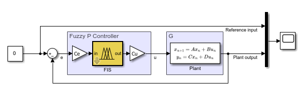

For this example, create a plant model.

A = [0.9995, 0.0100, 0.0001;
    -0.0020, 0.9995, 0.0106;
     0,      0,      0.9978];
B = [0, 0.002, 0.04]';
C = [2.3948, 0.3303, 2.2726];
D = 0;

Ts = 0.01;
G = ss(A,B,C,D,Ts);

The fuzzy controller uses a proportional (P) configuration with the following input and output scaling parameters Ce and Cu, both with a default value of 1.

To ensure global asymptotic stability, Lur'e systems require a static, sector‑bounded nonlinearity. Therefore, the fuzzy P controller must provide such a nonlinearity for the closed‑loop system to remain absolutely stable.

Load the initial fuzzy controller.

fis = readfis("fuzzypcontroller");

This fuzzy inference system (FIS) provides the following nonlinear, memory-less input-output mapping (control surface).

figure
gensurf(fis)

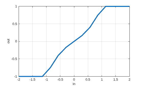
For this FIS, the original system has significant oscillations in the plant output signal.

sim(originalModel)
open_system(originalModel + "/output")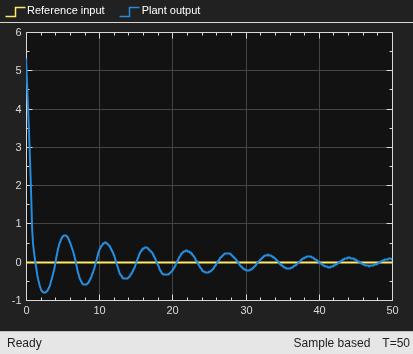

Close the output scope.

close_system(originalModel + "/output")

You can transform the model into a Lur'e system where the feedforward path contains the linear plant and the linear components of the fuzzy controller. The feedback path contains the nonlinear FIS. [2]

The FPAbsoluteStabilityLureSystem implements this system configuration.

transformedModel = "FPAbsoluteStabilityLureSystem";
open_system(transformedModel)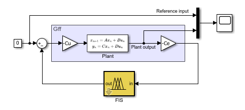

Here, the linear system in the feedforward path is:

Gff = (-Cu)*G*(-Ce);

To confirm that the plant output is the same for this system, simulate the model using the same initial FIS.

sim(transformedModel)
open_system(transformedModel + "/output")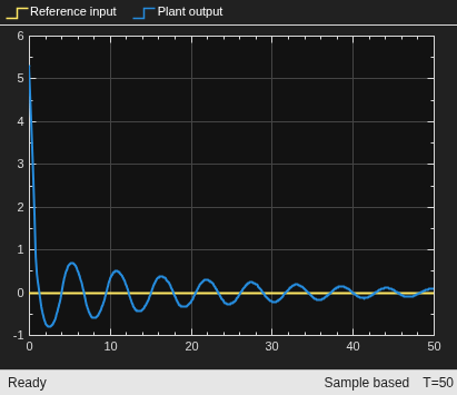

Close the output scope.

close_system(transformedModel + "/output")

FIS Sector Bounds

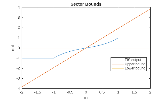
The FIS output is sector-bounded with straight lines passing through the origin, $$y=au$$ and $$y=bu$$. Here, $$a$$ is the slope of the lower bound and $$b$$ is the slope of the upper bound.

To plot the sector bounds, first generate input values across the FIS input range and evaluate the FIS at these points.

range = fis.Inputs(1).Range;
in = linspace(range(1),range(2),101)';
out = evalfis(fis,in);

Then, derive initial sector bounds based on the difference vectors of the input and output sequences.

m = diff(out)./diff(in);
a = min(m);
b = max(m);
figure
plotSectorBounds(in,out,a,b)

Conic Sector Index

The sector bounds define a conic sector where $$(y-au)(y-bu)<0$$, which you can parameterize as:

$${\left(\begin{array}{c}y\\ u\end{array}\right)}^{T}Q\left(\begin{array}{c}y\\ u\end{array}\right)<0,$$

where $$Q$$ is the conic sector matrix.

$$Q=\left[\begin{array}{cc}1& -\frac{a+b}{2}\\ -\frac{a+b}{2}& a\cdot b\end{array}\right]$$

Q = [1 -(a+b)/2;-(a+b)/2 a*b];

Calculate the conic sector index for this system. If the sector index is less than 1, then all output trajectories of Gff lie within the sector bounds of the fuzzy system, which satisfies the absolute stability condition.

Here:

• To analyze whether all I/O trajectories of linear system G lie in a particular sector, use H = [I;Gff].

• –Q is the conic sector for the nonlinear system in the feedback path of the transformed model.

H = [1;-Gff];
[RX,FX] = getSectorIndex(H,-Q)

RX = 
3.3299

FX = 
1.1353

Since the sector index RX is greater than 1, the control system does not satisfy the absolute stability condition. FX is the frequency at which the maximum sector index occurs.

You can plot the sector indices as a function of frequency.

figure
sectorplot(H,-Q,{0,FX})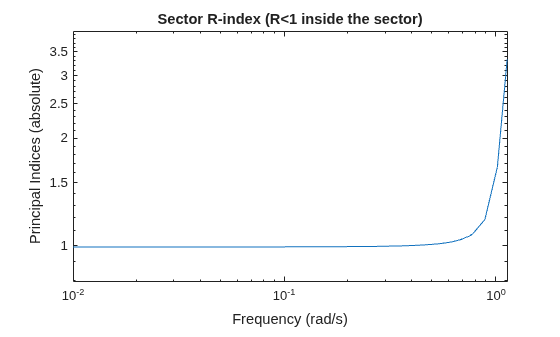

Update Sector Bounds to Improve Absolute Stability

To improve the absolute stability of the system, narrow the sector bounds. To do so, modify the FIS rules. For example, remove the output saturation from the FIS by modifying the parameters of the output membership functions.

fis = readfis("fuzzypcontrollernsb");
figure
gensurf(fis)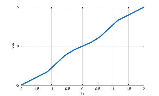

Compute and plot the sector bounds for the new FIS.

out = evalfis(fis,in);
m = diff(out)./diff(in);
a = min(m);
b = max(m);
figure
plotSectorBounds(in,out,a,b)

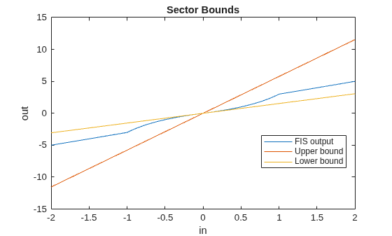
Calculate and plot the new sector index values.

Q = [1 -(a+b)/2;-(a+b)/2 a*b];
[RX,FX] = getSectorIndex(H,-Q)

RX = 
0.6037

FX = 
314.1593

figure
sectorplot(H,-Q,{0,FX})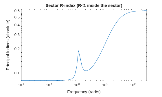

The sector index is now less than 1, satisfying the absolute stability condition.

To verify that the updated FIS produces a more stable system, simulate the original.

sim(originalModel)
open_system(originalModel + "/output")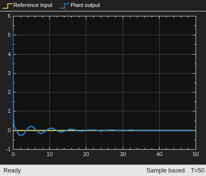

When using the updated FIS, the plant output is more stable with fewer oscillations.

Next Steps

• Extend this example for a fuzzy PD controller as described in [2].

• Tune fuzzy controller scaling parameters to optimize sector index values using Control System Tuner (Control System Toolbox) with a Conic Sector Goal (Control System Toolbox).

References

1. Xia, M., P. Gahinet, N. Abroug, C. Buhr, and E. Laroche. "Sector Bounds in Stability Analysis and Control Design". International Journal of Robust and Nonlinear Control 30, no. 18 (December 2020): 7857–82.

2. R. Katoh, T. Tamashita, and S. Singh. "Stability analysis of control system having PD type of fuzzy controller". Fuzzy Sets and Systems 74 (1995) 321-334.

Local Functions

function plotSectorBounds(in,out,a,b)
% Plot sector bounds.
lowerBound = a*in;
upperBound = b*in;
plot(in,out)
hold on
plot(in,upperBound)
plot(in,lowerBound)
hold off
xlabel("in")
ylabel("out")
title("Sector Bounds")
legend("FIS output","Upper bound","Lower bound",Location="best")
end