Optimize an Unfolded CORDIC Design for ASIC Clock Constraints by Using Improved Adaptive Pipelining (Tech Preview)
R2026bNote
Improved adaptive pipelining is a tech preview in R2026b. The behavior, implementation, and interfaces might change before general release. Do not use the optimization in production designs.
To enable the improved adaptive pipelining optimization, run this command at the start of each MATLAB session:
matlab.internal.feature("GlobalAdaptivePipelining",1);To send feedback about improved adaptive pipelining, email the development team.
This example shows how to use improved adaptive pipelining to meet a 125 MHz ASIC clock constraint on an unfolded CORDIC design. Adaptive pipelining is an optimization in HDL Coder that adds pipeline registers to multipliers to achieve greater performance. Improved adaptive pipelining optimizes the design under test (DUT) by adding pipeline registers according to a target device or architecture and frequency.
In high-speed ASIC systems, such as 5G baseband processors or radar signal processors, CORDIC designs compute the phase rotations at a system clock rate of hundreds of megahertz. An unfolded CORDIC design outputs one result per clock cycle, but has a deep combinational path that violates timing. Improved adaptive pipelining achieves the target frequency by analyzing this path and inserts pipeline registers. The resulting pipelining adds latency but sustains full throughput of one result per clock cycle after the initial fill, and downstream blocks can account for the fixed latency.
Prerequisites
Improved adaptive pipelining is a tech preview in R2026b. Enable it by using this command.
matlab.internal.feature("GlobalAdaptivePipelining",1);Open Model
The model implements an unfolded, parallel, eight-iteration CORDIC sine and cosine function by using a single MATLAB Function block. Unlike iterative CORDIC architectures, which reuse one rotation unit across multiple clock cycles, the unfolded architecture chains all eight rotation stages in series, which produces one result per clock cycle with no feedback loops.
This architecture is typical of CORDIC designs in applications such as correcting carrier frequency offset in 5G NR baseband at the sample rate, performing digital beamforming with per-element phase rotation in radar, and implementing numerically controlled oscillators and IQ demodulation in software-defined radios.
To eliminate the final multiplier, this CORDIC architecture uses gain pre-compensation, which means that it initializes instead of .
model = "hdlcordic_unfolded";
open_system(model);
The unfolded architecture computes sine and cosine through eight cascaded shift-and-add micro-rotation stages.
Because all eight stages execute in a single clock cycle, the critical path passes through all eight rotation stages and the quadrant correction logic.
open_system(model + "/Cordic_Unfolded");Simulate and Verify Functional Correctness
Simulate the model to verify that the CORDIC outputs match the floating-point reference. The test bench sweeps the input angles from 0 to 359 degrees and compares them against the MATLAB cosd and sind functions.
out = sim(model);
Configure Model for ASIC Synthesis Targeting
Critical path estimation (CPE) relies on timing databases that characterize the cell delays for a specified target device, speed grade, and synthesis tool. HDL Coder™ ships with a timing database for the tutorial.lib chip family. To use it, set the SynthesisToolChipFamily model configuration parameter to tutorial.lib, a 45 nm standard cell library that is compatible with Cadence® Genus™ synthesis. To target a different device, speed grade, or library node, use the genhdltdb function to generate a timing database for that configuration.
For this example, set the SynthesisTool model configuration parameter to Cadence Genus. To optimize the MATLAB Function blocks in the model, set the Architecture HDL block property on all MATLAB Function blocks to MATLAB Datapath.
hdlset_param(model,SynthesisTool="Cadence Genus");
hdlset_param(model,SynthesisToolChipFamily="tutorial.lib");

mfbBlocks = find_system(model + "/Cordic_Unfolded",SFBlockType="MATLAB Function");
for k = 1:numel(mfbBlocks)
    hdlset_param(mfbBlocks{k},Architecture="MATLAB Datapath");
end
Generate Baseline HDL Code Without Pipelining
Establish the baseline critical path of the model by generating HDL code targeting 125 MHz without adaptive pipelining. The 125 MHz target represents a typical system clock for a 45 nm ASIC.
hdlset_param(model,HDLSubsystem=model + "/Cordic_Unfolded");
hdlset_param(model,TargetDirectory=fullfile(pwd,"hdlsrc_baseline"));
hdlset_param(model,TargetFrequency=125);
hdlset_param(model,CriticalPathEstimation="on");
hdlset_param(model,AdaptivePipelining="off");
hdlset_param(model,ResourceReport="on");
hdlset_param(model,GenerateModel="on");

hdlset_param("hdlcordic_unfolded/Cordic_Unfolded",InputPipeline=1);
hdlset_param("hdlcordic_unfolded/Cordic_Unfolded",OutputPipeline=1);

evalc('makehdl(model + "/Cordic_Unfolded")');
Run Baseline Synthesis with Cadence Genus
Use the hdlcoder.runWorkflow function to run Cadence Genus synthesis on the baseline HDL code. This function validates the CPE timing estimate against actual post-synthesis results. This code runs only when your operating system is Linux, because Cadence Genus requires Linux.
genusAvailable = isunix && ~isempty(hdlsetuptoolpath('ToolName','Cadence Genus'));
if genusAvailable
    hdlset_param(model,SynthesisToolChipFamily="");
    hWC = hdlcoder.WorkflowConfig('SynthesisTool','Cadence Genus','TargetWorkflow','Generic ASIC/FPGA');
    hWC.ProjectFolder = 'hdl_prj_baseline';
    hWC.RunTaskGenerateRTLCodeAndTestbench = false;
    hWC.RunTaskCreateProject = true;
    hWC.RunTaskPerformLogicSynthesis = true;
    hWC.validate;
    hdlcoder.runWorkflow(model + "/Cordic_Unfolded",hWC);
    hdlset_param(model,SynthesisToolChipFamily="tutorial.lib");
end
Examine Baseline Results
Open the code generation report to examine the estimated critical path and resource usage. Cadence Genus writes the post-synthesis QOR report to hdl_prj_baseline/genus_prj/reports/Cordic_Unfolded_qor.txt. To see the combinational critical path, run the hdlsrc_baseline\hdlcordic_unfolded\criticalPathEstimated.m script.
web(fullfile(pwd,"hdlsrc_baseline","hdlcordic_unfolded","html","index.html"));
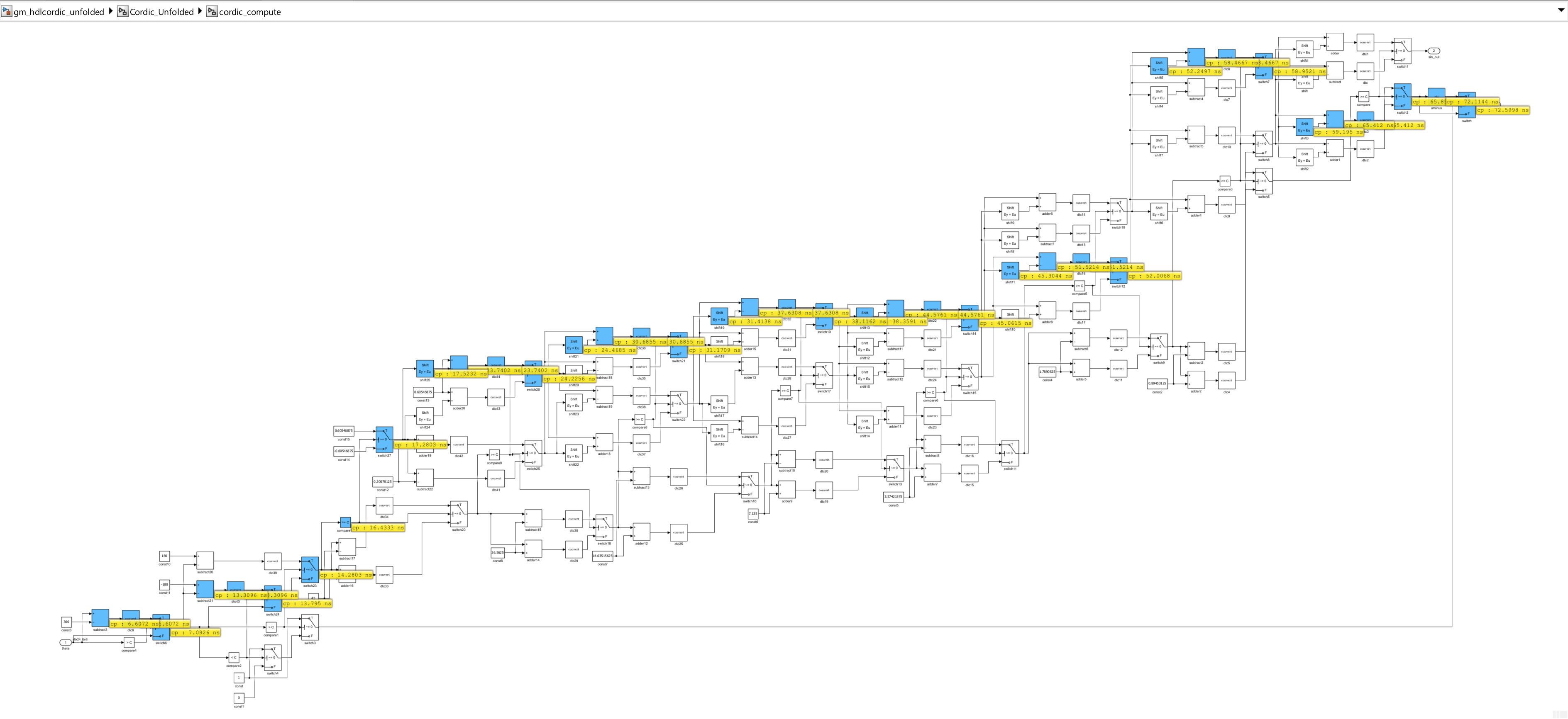
The baseline design is purely combinational, with zero registers and zero latency. The datapath includes only adders and multiplexers that implement the shift-and-add operations. Without adaptive pipelining, meeting 125 MHz manually requires identifying the cut points in the eight-stage cascade and inserting pipeline registers between stages, a trial-and-error process that depends on detailed timing analysis at each step.
Enable Improved Adaptive Pipelining
To preserve the baseline output, change the code generation directory to a new folder. Set the AdaptivePipelining model configuration parameter to on, restore SynthesisToolChipFamily to tutorial.lib, and regenerate the HDL code.
hdlset_param(model,TargetDirectory=fullfile(pwd,"hdlsrc_gap"));
hdlset_param(model,SynthesisToolChipFamily="tutorial.lib");
hdlset_param(model,AdaptivePipelining="on");

evalc('makehdl(model + "/Cordic_Unfolded")');
Run Adaptive Pipelining Synthesis with Cadence Genus
Run Cadence Genus synthesis on the DUT to confirm that the design meets the 125 MHz target.
if genusAvailable
    hdlset_param(model,SynthesisToolChipFamily="");
    hWC = hdlcoder.WorkflowConfig('SynthesisTool','Cadence Genus','TargetWorkflow','Generic ASIC/FPGA');
    hWC.ProjectFolder = 'hdl_prj_gap';
    hWC.RunTaskGenerateRTLCodeAndTestbench = false;
    hWC.RunTaskCreateProject = true;
    hWC.RunTaskPerformLogicSynthesis = true;
    hWC.validate;
    hdlcoder.runWorkflow(model + "/Cordic_Unfolded",hWC);
    hdlset_param(model,SynthesisToolChipFamily="tutorial.lib");
end
Examine Improved Adaptive Pipelining Results
Open the code generation report to examine the improved adaptive pipelining CPE results. To see the critical path, run the hdlsrc_gap\hdlcordic_unfolded\criticalPathEstimated.m script.
web(fullfile(pwd,"hdlsrc_gap","hdlcordic_unfolded","html","index.html"));
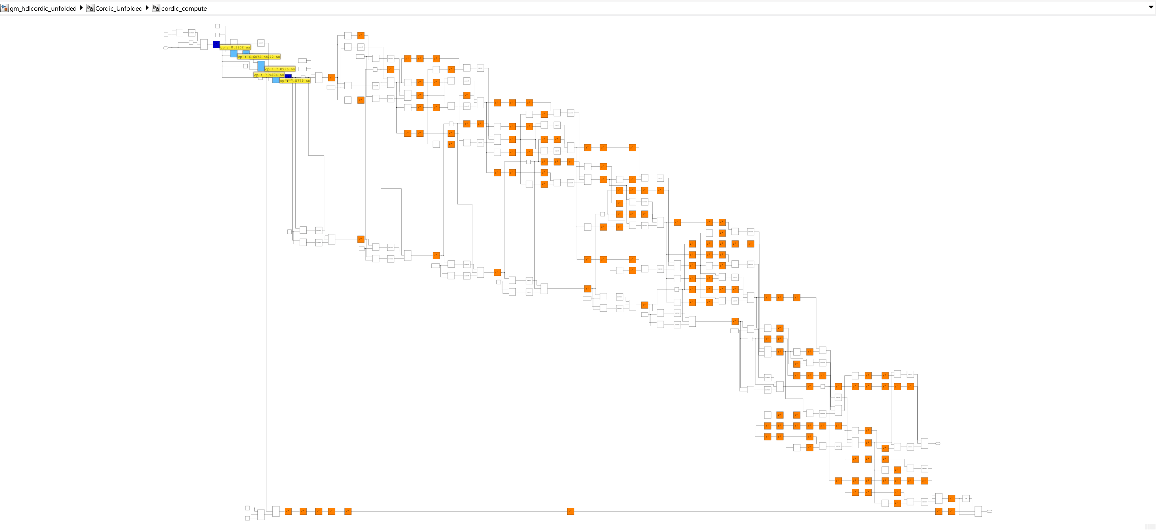
Compare Baseline and Improved Adaptive Pipelining Results
This table compares the CPE estimates for the baseline and improved adaptive pipelining results and the synthesis results from Cadence Genus.
comparisonTable = table([72.21; 7.92],[14; 126],[15.2; 6.675],[65.79; 149.8],[0; 19],[0; 122],[7977.5; 17710], ...
    VariableNames=["CPE Critical Path (ns)", "CPE Max Freq (MHz)", ...
    "Synthesis Critical Path (ns)", "Synthesis Max Freq (MHz)", ...
    "Latency (cycles)", "Registers", "Area (cells)"], ...
    RowNames=["Baseline", "Adaptive"]);
disp(comparisonTable);
                CPE Critical Path (ns)    CPE Max Freq (MHz)    Synthesis Critical Path (ns)    Synthesis Max Freq (MHz)    Latency (cycles)    Registers    Area (cells)
                ______________________    __________________    ____________________________    ________________________    ________________    _________    ____________

    Baseline            72.21                     14                        15.2                         65.79                      0                0          7977.5
    Adaptive             7.92                    126                       6.675                         149.8                     19              122           17710
Improved adaptive pipelining met the target frequency by reducing the critical path from approximately 72 ns to approximately 8 ns, which resulted in a CPE estimate of 126 MHz. This is an approximately nine times improvement from the baseline of 14 MHz. Cadence Genus synthesis confirms that the post-synthesis critical path is 6.675 ns, or 149.8 MHz, which confirms that the design meets the 125 MHz target. The baseline synthesis critical path of 15.2 ns, or 65.79 MHz, confirms that the unpipelined design cannot meet the 125 MHz target without pipelining.
Improved adaptive pipelining inserts 19 pipeline stages with 122 registers, which is the minimum depth needed to meet the constraint. The area increased from 7977.5 cells in the baseline result to 17710 cells due to the added pipeline registers. These additions resulted in a 2.2 times area increase for a nine times frequency improvement. The combinational logic does not change because improved adaptive pipelining does not restructure the datapath or add logic.
Adapt to Another ASIC Target
To target a different technology node, change the timing database and target frequency of the model. For example, to target 500 MHz on a 7 nm node, generate a 7 nm timing database with genhdltdb and set TargetFrequency to 500.

