imfill

Fill image regions and holes

Syntax

BW2 = imfill(BW,locations)

BW2 = imfill(BW,locations,conn)

BW2 = imfill(BW,"holes")

BW2 = imfill(BW,conn,"holes")

I2 = imfill(I)

I2 = imfill(I,conn)

BW2 = imfill(BW)

BW2 = imfill(BW,0,conn)

[BW2, locations_out] = imfill(BW)

Description

Binary Images

BW2 = imfill(BW,locations) performs a flood-fill operation on background pixels of the input binary image BW, starting from the points specified in locations.

BW2 = imfill(BW,locations,conn) fills the area defined by locations, where conn specifies the connectivity.

BW2 = imfill(BW,"holes") fills holes in the input binary image BW. In this syntax, a hole is a set of background pixels that cannot be reached by filling in the background from the edge of the image.

BW2 = imfill(BW,conn,"holes") fills holes in the binary image BW, where conn specifies the connectivity.

Grayscale Images

I2 = imfill(I) fills holes in the grayscale image I. In this syntax, a hole is defined as an area of dark pixels surrounded by lighter pixels.

I2 = imfill(I,conn) fills holes in the grayscale image I, where conn specifies the connectivity.

Interactive Behavior

BW2 = imfill(BW) displays the binary image BW on the screen and lets you define the region to fill by selecting points interactively with the mouse. To use this syntax, BW must be a 2-D image.

Press Backspace or Delete to remove the previously selected point. Shift-click, right-click, or double-click to select a final point and start the fill operation. Press Return to finish the selection without adding a point.

BW2 = imfill(BW,0,conn) lets you override the default connectivity as you interactively specify locations.

[BW2, locations_out] = imfill(BW) returns the locations of points selected interactively in locations_out. To use this syntax, BW must be a 2-D image.

Examples

Fill Image from Specified Starting Point

Create an 8-by-8 binary image.

BW1 = logical([1 0 0 0 0 0 0 0
               1 1 1 1 1 0 0 0
               1 0 0 0 1 0 1 0
               1 0 0 0 1 1 1 0
               1 1 1 1 0 1 1 1
               1 0 0 1 1 0 1 0
               1 0 0 0 1 0 1 0
               1 0 0 0 1 1 1 0]);

Perform a flood-fill operation starting at the location BW1(3,3). Specify the third input argument as 4 to fill the image using 4-connectivity. The operation fills the hole in the top-left region of the image.

BW2 = imfill(BW1,[3 3],4)

BW2 = 8×8 logical array

   1   0   0   0   0   0   0   0
   1   1   1   1   1   0   0   0
   1   1   1   1   1   0   1   0
   1   1   1   1   1   1   1   0
   1   1   1   1   0   1   1   1
   1   0   0   1   1   0   1   0
   1   0   0   0   1   0   1   0
   1   0   0   0   1   1   1   0

Perform a flood-fill operation from the same pixel, this time using 8-connectivity. The filled area now also includes the hole in the bottom-right region of the image.

BW3 = imfill(BW1,[3 3],8)

BW3 = 8×8 logical array

   1   0   0   0   0   0   0   0
   1   1   1   1   1   0   0   0
   1   1   1   1   1   0   1   0
   1   1   1   1   1   1   1   0
   1   1   1   1   1   1   1   1
   1   0   0   1   1   1   1   0
   1   0   0   0   1   1   1   0
   1   0   0   0   1   1   1   0

Fill Holes in a Binary Image

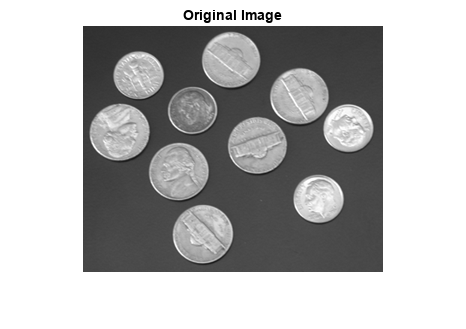
Read image into workspace.

I = imread('coins.png');
figure
imshow(I)
title('Original Image')

Convert image to binary image.

BW = imbinarize(I);
figure
imshow(BW)
title('Original Image Converted to Binary Image')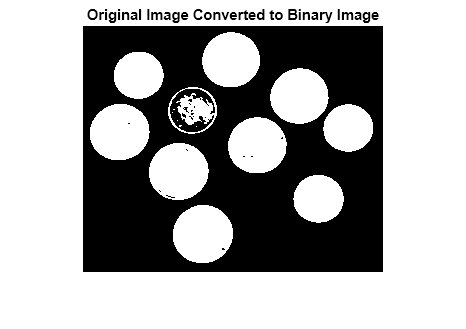

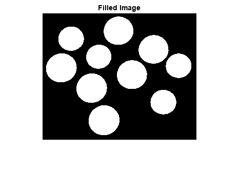
Fill holes in the binary image and display the result.

BW2 = imfill(BW,'holes');
figure
imshow(BW2)
title('Filled Image')

Fill Holes in a Grayscale Image

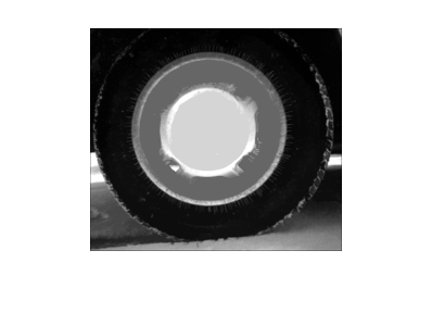
I = imread('tire.tif');
I2 = imfill(I);
figure, imshow(I), figure, imshow(I2)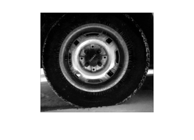

Input Arguments

BW — Binary image

logical array

Binary image, specified as a logical array of any dimension.

Data Types: logical

locations — Indices identifying pixel locations

p-by-ndims(BW) matrix of positive integers | p-element column vector of positive integers

Indices identifying pixel locations, specified as one of these options.

• To specify p locations using their subscript indices, specify a p-by-ndims(BW) matrix of positive integers. Here, ndims(BW) is the number of dimensions in the input image, and each row contains the subscript indices for one location.

• To specify p locations using their linear indices, specify a p-element column vector of positive integers.

Example: [3 4] specifies one location within a 2-D input image with the row and column indices (3, 4).

Example: [2 2 2; 4 5 6] specifies two locations within a 3-D input image with subscript indices (2, 2, 2) and (4, 5, 6)

Example: 2 specifies a single location corresponding to the linear index 2.

Example: [2; 8; 16] specifies three locations corresponding to the linear indices 2, 8, and 16.

Data Types: double

conn — Pixel connectivity

4 | 8 | 6 | 18 | 26 | 3-by-3-by- ... -by-3 matrix of 0s and 1s

Pixel connectivity, specified as one of the values in this table. The default connectivity is 4 for 2-D images, and 6 for 3-D images.

Value	Meaning
Two-Dimensional Connectivities
4	Pixels are connected if their edges touch. The neighborhood of a pixel are the adjacent pixels in the horizontal or vertical direction.	Current pixel is shown in gray.
8	Pixels are connected if their edges or corners touch. The neighborhood of a pixel are the adjacent pixels in the horizontal, vertical, or diagonal direction.	Current pixel is shown in gray.
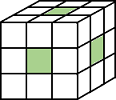
Three-Dimensional Connectivities
6	Pixels are connected if their faces touch. The neighborhood of a pixel are the adjacent pixels in: One of these directions: in, out, left, right, up, and down	Current pixel is shown in gray.
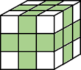
18	Pixels are connected if their faces or edges touch. The neighborhood of a pixel are the adjacent pixels in: One of these directions: in, out, left, right, up, and down A combination of two directions, such as right-down or in-up	Current pixel is center of cube.
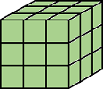
26	Pixels are connected if their faces, edges, or corners touch. The neighborhood of a pixel are the adjacent pixels in: One of these directions: in, out, left, right, up, and down A combination of two directions, such as right-down or in-up A combination of three directions, such as in-right-up or in-left-down	Current pixel is center of cube.

For higher dimensions, imfill uses the default value conndef(ndims(BW),"minimal").

Connectivity can also be defined in a more general way for any dimension by specifying a 3-by-3-by- ... -by-3 matrix of 0s and 1s. The 1-valued elements define neighborhood locations relative to the center element of conn. Note that conn must be symmetric about its center element. See Specifying Custom Connectivities for more information.

Data Types: double | logical

I — Grayscale image

numeric array

Grayscale image, specified as a numeric array of any dimension.

Data Types: single | double | int8 | int16 | int32 | int64 | uint8 | uint16 | uint32 | uint64

Output Arguments

BW2 — Filled binary image

logical array

Filled binary image, returned as logical array.

locations_out — Linear indices of pixel locations

numeric vector | numeric matrix

Linear indices of pixel locations, returned as a numeric vector or matrix.

I2 — Filled grayscale image

numeric array

Filled grayscale image, returned as a numeric array.

Algorithms

imfill uses an algorithm based on morphological reconstruction [1].

References

[1] Soille, P., Morphological Image Analysis: Principles and Applications, Springer-Verlag, 1999, pp. 173–174.

Extended Capabilities

C/C++ Code Generation

Generate C and C++ code using MATLAB® Coder™.

Usage notes and limitations:

• imfill supports the generation of C code (requires MATLAB^® Coder™). Note that if you choose the generic MATLAB Host Computer target platform, imfill generates code that uses a precompiled, platform-specific shared library. Use of a shared library preserves performance optimizations but limits the target platforms for which code can be generated. For more information, see Types of Code Generation Support in Image Processing Toolbox.

• The optional input arguments, conn and "holes", must be compile-time constants.

• Input argument "holes" is not supported, if the input is a binary image.

• imfill supports up to 3-D inputs only. (No N-D support.)

• The interactive syntaxes to select points are not supported. For example, the syntax imfill(BW,0,CONN) is not supported.

• With the locations input argument, once you select a format at compile time, you cannot change it at run time. However, the number of points in locations can be varied at run time.

Thread-Based Environment

Run code in the background using MATLAB® backgroundPool or accelerate code with Parallel Computing Toolbox™ ThreadPool.

This function fully supports thread-based environments. For more information, see Run MATLAB Functions in Thread-Based Environment.

GPU Arrays

Accelerate code by running on a graphics processing unit (GPU) using Parallel Computing Toolbox™.

Usage notes and limitations:

• Inputs must be 2-D, supporting only the 2-D connectivities (4 and 8).

• The interactive syntaxes to select points are not supported. For example, the syntax imfill(BW) is not supported.

For more information, see Image Processing on a GPU.

Version History

Introduced before R2006a

R2022b: Support for thread-based environments

imfill now supports thread-based environments.