regionprops
Measure properties of image regions
Syntax
Description
The regionprops function measures properties such as area,
centroid, and bounding box, for each object (connected component) in an image.
regionprops supports both contiguous regions
and discontiguous regions.
regionprops finds unique objects in binary images using 8-connected
neighborhoods for 2-D images and maximal connectivity for higher dimension images. For more
information, see Pixel Connectivity. To find objects using other
types of connectivity, use bwconncomp to create the connected components,
and then pass the result to regionprops using the CC
argument instead.
Note
To measure properties of objects in a 3-D volumetric image, consider using regionprops3
instead. Although regionprops can accept 3-D images,
regionprops3 supports more statistics for 3-D images.
When you call the regionprops function, you can omit the
properties argument, in which case the function returns the
"Area", "Centroid", and
"BoundingBox" measurements.
stats = regionprops(BW,properties)BW.
stats = regionprops(CC,properties)CC.
stats = regionprops(L,properties)L.
stats = regionprops(outputFormat,___)outputFormat argument.
Examples
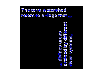
Read a binary image into workspace.
BW = imread("text.png");Calculate centroids for connected components in the image using regionprops. The regionprops function returns the centroids in a structure array.
s = regionprops(BW,"centroid");Store the x- and y-coordinates of the centroids into a two-column matrix.
centroids = cat(1,s.Centroid);
Display the binary image with the centroid locations superimposed.
imshow(BW)
hold on
plot(centroids(:,1),centroids(:,2),"m.")
hold off
Estimate the center and radii of circular objects in an image and use this information to plot circles on the image. In this example, regionprops returns the measured region properties in a table.
Read an image into workspace.
a = imread("circlesBrightDark.png");Turn the input image into a binary image.
bw = a < 50;
imshow(bw)
title("Image with Circles")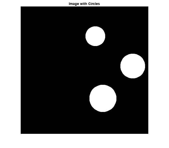
Calculate properties of regions in the image and return the data in a table.
stats = regionprops("table",bw,"Centroid", ...
    "MajorAxisLength","MinorAxisLength")
stats=3×3 table
        Centroid        MajorAxisLength    MinorAxisLength
    ________________    _______________    _______________

       300       120        79.517             79.517
    330.29    369.92        109.49              108.6
       450       240        99.465             99.465
Get centers and radii of the circles.
centers = stats.Centroid;
diameters = mean([stats.MajorAxisLength stats.MinorAxisLength],2);
radii = diameters/2;
Plot the circles.
hold on
viscircles(centers,radii)
ans =
Group with properties:
Children: [2×1 Line]
Visible: on
HitTest: on
Show all properties
hold off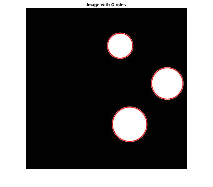
Read a binary image and detect the connected components.
BW = imread("text.png");
CC = bwconncomp(BW);
Measure the area of each connected component and return the results as a table.
p = regionprops("table",CC,"Area");
Create a binary image that contains only the 2nd through 10th largest connected components. Display the result.
[~,idx] = sort(p.Area,"descend");
BWfilt = cc2bw(CC,ObjectsToKeep=idx(2:10));
imshow(BWfilt)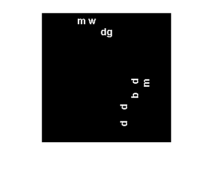
Read a grayscale image of grains of rice, then convert the image to binary.
I = imread("rice.png");
BW = imbinarize(I);
imshow(BW)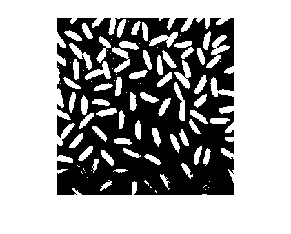
Measure the area and bounding box of each region.
CC = bwconncomp(BW);
stats = regionprops("table",CC,"Area","BoundingBox");
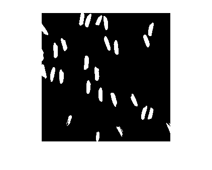
Select regions for whom these conditions apply:
The area is greater than 50 pixels
The bounding box is less than 15 pixels wide and is greater than or equal to 20 pixels tall.
area = stats.Area;
bbox = stats.BoundingBox;
selection = (area > 50) & (bbox(:,3) < 15) & (bbox(:,4) >= 20);
BW2 = cc2bw(CC,ObjectsToKeep=selection);
Display the filtered image.
imshow(BW2)
Input Arguments
Binary image, specified as a logical array of any dimension.
regionprops sorts the objects in the binary image from left to
right based on the top-left extremum of each component. When multiple
objects have the same horizontal position, the function then sorts those objects from
top to bottom, and again along any higher dimensions. regionprops
returns the measured properties, stats, in the same order as the
sorted objects.
Data Types: logical
Connected components, specified as a structure with four fields. You can get a
connected components structure by using the bwconncomp or bwpropfilt function.
| Field | Description |
|---|---|
Connectivity | Connectivity of the connected components (objects) |
ImageSize | Size of the binary image |
NumObjects | Number of connected components (objects) in the binary image |
PixelIdxList | 1-by-NumObjects cell array where the
k-th element in the cell array is a vector containing
the linear indices of the pixels in the k-th
object |
Data Types: struct
Label image, specified as one of the following.
A numeric array of any dimension. Pixels labeled
0are the background. Pixels labeled1make up one object; pixels labeled2make up a second object; and so on.regionpropstreats negative-valued pixels as background and rounds down input pixels that are not integers. You can get a numeric label image from labeling functions such aswatershedorlabelmatrix.A categorical array. Each category corresponds to a different region.
Data Types: single | double | int8 | int16 | int32 | uint8 | uint16 | uint32 | categorical
Type of measurement, specified as a comma-separated list of string scalars or character
vectors, an array of string scalars, a cell array of character vectors, or as
"all" or "basic".
If you specify
"all", thenregionpropscomputes all the shape measurements and, for grayscale images, the pixel value measurements as well.If you specify
"basic", thenregionpropscomputes only the"Area","Centroid", and"BoundingBox"measurements.
The following tables list all the properties that provide shape measurements. The properties listed in the Pixel Value Measurements table are valid only when you specify a grayscale image.
Shape Measurements
| Property Name | Description | N-D Support | GPU Support | Code Generation | ||||||||
|---|---|---|---|---|---|---|---|---|---|---|---|---|
"Area" | Number of To find
the equivalent to the area of a 3-D volume, use the
| Yes | Yes | Yes | ||||||||
"BoundaryCoordinates" (since R2026a) | Coordinates of pixels on the exterior boundary of the region. The
coordinates match the result of calling the This property is supported only for 2-D binary images,
| 2-D only | No | Yes | ||||||||
"BoundingBox" | Position and size of the smallest box containing the region, returned as a
1-by-(2*Q) vector, where Q is the
image dimensionality. The first Q elements are the
coordinates of the minimum corner of the box. The second Q
elements are the size of the box along each dimension. For example, a 2-D
bounding box with value | Yes | Yes | Yes | ||||||||
"Centroid" | Center of mass of the region, returned as a 1-by-Q vector, where
Q is the image dimensionality. The first element of
This figure illustrates the centroid and bounding box for a discontiguous region. The region consists of the white pixels. The green box is the bounding box, and the red dot is the centroid.
| Yes | Yes | Yes | ||||||||
"Circularity" | Roundness of objects, returned as a structure with field
The maximum circularity value is 1. The input
must be a label matrix or binary image with contiguous regions. If the image
contains discontiguous regions, | 2-D only | No | Yes | ||||||||
"ConvexArea" | Number of pixels in ConvexImage, returned as a scalar. | 2-D only | No | No | ||||||||
"ConvexHull" | Smallest convex polygon that can contain the region, returned as a p-by-2 matrix. Each row of the matrix contains the x- and y-coordinates of one vertex of the polygon. | 2-D only | No | No | ||||||||
"ConvexImage" | Image that specifies the convex hull, with all pixels within the hull filled in (set to
on), returned as a binary image. The image is the size of
the bounding box of the region. For pixels that the boundary of the hull passes
through, regionprops uses the algorithm described by Classify Pixels That Are Partially Enclosed by ROI. | 2-D only | No | No | ||||||||
"Eccentricity" | Eccentricity of the ellipse that has the same second-moments as the region, returned as a scalar. The eccentricity is the ratio of the distance between the foci of the ellipse and its major axis length. The value is between 0 and 1. (0 and 1 are degenerate cases. An ellipse whose eccentricity is 0 is actually a circle, while an ellipse whose eccentricity is 1 is a line segment.) | 2-D only | Yes | Yes | ||||||||
"EquivDiameter" | Diameter of a circle with the same area as the region, returned as a scalar. Computed as
sqrt(4*Area/pi). | 2-D only | Yes | Yes | ||||||||
"EulerNumber" | Number of objects in the region minus the number of holes in those objects, returned as a
scalar. This property is supported only for 2-D label matrices.
regionprops uses 8-connectivity to compute the Euler
number (also known as the Euler characteristic). To learn more about
connectivity, see Pixel Connectivity. | 2-D only | No | Yes | ||||||||
"Extent" | Ratio of pixels in the region to pixels in the total bounding box, returned as a scalar.
regionprops calculates this property as the
Area divided by the area of the bounding box. | 2-D only | Yes | Yes | ||||||||
"Extrema" | Extrema points in the region, returned as an 8-by-2 matrix. Each row of the matrix
contains the x- and y-coordinates of
one of the points. The format of the vector is This figure illustrates the extrema of two
different regions. In the region on the left, each extrema point is distinct.
For the region on the right, certain extrema points (such as
| 2-D only | Yes | Yes | ||||||||
"FilledArea" | Number of on pixels in FilledImage, returned as a
scalar. | Yes | No | Yes | ||||||||
"FilledImage" | Image the same size as the bounding box of the region, returned as a binary array. The
| Yes | No | Yes | ||||||||
"Image" | Image the same size as the bounding box of the region, returned as a binary array. The
on pixels correspond to the region, and all other pixels
are off. | Yes | Yes | Yes | ||||||||
"MajorAxisLength" | Length (in pixels) of the major axis of the ellipse that has the same normalized second central moments as the region, returned as a scalar. | 2-D only | Yes | Yes | ||||||||
"MaxFeretProperties" | Feret properties that include maximum Feret diameter, its relative angle, and coordinate values, returned as a structure with fields:
The input can be a binary image, connected component, or a label matrix. | 2-D only | No | No | ||||||||
"MinFeretProperties" | Feret properties that include minimum Feret diameter, its relative angle, and coordinate values, returned as a structure with fields:
The input can be a binary image, a connected component, or a label matrix. | 2-D only | No | No | ||||||||
"MinorAxisLength" | Length (in pixels) of the minor axis of the ellipse that has the same normalized second central moments as the region, returned as a scalar. | 2-D only | Yes | Yes | ||||||||
"Orientation" | Angle between the x-axis and the major axis of the ellipse that has the same second-moments as the region, returned as a scalar. The value is in degrees, ranging from -90 degrees to 90 degrees. This figure illustrates the axes and orientation of the ellipse. The left side of the figure shows an image region and its corresponding ellipse. The right side shows the same ellipse with the solid blue lines representing the axes. The red dots are the foci. The orientation is the angle between the horizontal dotted line and the major axis.
| 2-D only | Yes | Yes | ||||||||
"Perimeter" | Distance around the boundary of the region returned as a scalar.
| 2-D only | No | Yes | ||||||||
"PixelIdxList" | Linear indices of the pixels in the region, returned as a p-element vector. | Yes | Yes | Yes | ||||||||
"PixelList" | Locations of pixels in the region, returned as a p-by-Q
matrix. Each row of the matrix has the form [x y z ...] and
specifies the coordinates of one pixel in the region. | Yes | Yes | Yes | ||||||||
"Solidity" | Proportion of the pixels in the convex hull that are also in the region, returned as a
scalar. The solidity is calculated as
| 2-D only | No | No | ||||||||
"SubarrayIdx" | Elements of L inside the object bounding box, returned as a cell array
that contains indices such that L(idx{:}) extracts the
elements. | Yes | Yes | No |

The pixel value measurement properties in the following table
are valid only when you specify a grayscale image, I.
Pixel Value Measurements
| Property Name | Description | N-D Support | GPU Support | Code Generation |
|---|---|---|---|---|
"MaxIntensity" | Value of the pixel with the greatest intensity in the region, returned as a scalar. | Yes | Yes | Yes |
"MeanIntensity" | Mean of all the intensity values in the region, returned as a scalar. | Yes | Yes | Yes |
"MinIntensity" | Value of the pixel with the lowest intensity in the region, returned as a scalar. | Yes | Yes | Yes |
"PixelValues" | Number of pixels in the region, returned as a p-by-1 vector, where p is the number of pixels in the region. Each element in the vector contains the value of a pixel in the region. | Yes | Yes | Yes |
"WeightedCentroid" | Center of the region based on location and intensity value, returned as a
p-by-Q vector of coordinates. The first
element of WeightedCentroid is the horizontal coordinate (or
x-coordinate) of the weighted centroid. The second
element is the vertical coordinate (or y-coordinate). All
other elements of WeightedCentroid are in order of dimension. | Yes | Yes | Yes |
Data Types: char | string | cell
Output format of the measurement values stats, specified as
either of the following values.
| Value | Description |
|---|---|
"struct" | Returns an array of structures with length equal to the number of objects
in BW,
max(. The fields of the
structure array denote different properties for each region, as specified by
properties. |
"table" | Returns a |
Data Types: char | string
Output Arguments
More About
Tips
regionpropstakes advantage of intermediate results when computing related measurements. Therefore, it is fastest to compute all the desired measurements in a single call toregionprops.Most of the measurements take little time to compute. However, these measurements can take longer, depending on the number of regions in
L:"ConvexHull""ConvexImage""ConvexArea""FilledImage"
The
cc2bwfunction is useful for creating a binary image containing only a subset of objects or regions that meet certain criteria.