Main Content

cumtrapz

Cumulative trapezoidal numerical integration

Description

example

Q = cumtrapz(Y) computes the approximate cumulative integral of Y via the trapezoidal method with unit spacing. The size of Y determines the dimension to integrate along:

  • If Y is a vector, then cumtrapz(Y) is the cumulative integral of Y.

  • If Y is a matrix, then cumtrapz(Y) is the cumulative integral over each column.

  • If Y is a multidimensional array, then cumtrapz(Y) integrates over the first dimension whose size does not equal 1.

example

Q = cumtrapz(X,Y) integrates Y with respect to the coordinates or scalar spacing specified by X.

  • If X is a vector of coordinates, then length(X) must be equal to the size of the first dimension of Y whose size does not equal 1.

  • If X is a scalar spacing, then cumtrapz(X,Y) is equivalent to X*cumtrapz(Y).

example

Q = cumtrapz(___,dim) integrates along the dimension dim using any of the previous syntaxes. You must specify Y, and optionally can specify X. If you specify X, then it can be a scalar or a vector with length equal to size(Y,dim). For example, if Y is a matrix, then cumtrapz(X,Y,2) cumulatively integrates each row of Y.

Examples

collapse all

Calculate the cumulative integral of a vector where the spacing between data points is 1.

Create a numeric vector of data.

Y = [1 4 9 16 25];

Y contains function values for f(x)=x2 in the domain [1 5].

Use cumtrapz to integrate the data with unit spacing.

Q = cumtrapz(Y)
Q = 1×5

         0    2.5000    9.0000   21.5000   42.0000

This approximate integration yields a final value of 42. In this case, the exact answer is a little less, 4113. The cumtrapz function overestimates the value of the integral because f(x) is concave up.

Calculate the cumulative integral of a vector where the spacing between data points is uniform, but not equal to 1.

Create a domain vector.

X = 0:pi/5:pi;

Calculate the sine of X.

Y = sin(X');

Cumulatively integrate Y using cumtrapz. When the spacing between points is constant, but not equal to 1, an alternative to creating a vector for X is to specify the scalar spacing value. In that case, cumtrapz(pi/5,Y) is the same as pi/5*cumtrapz(Y).

Q = cumtrapz(X,Y)
Q = 6×1

         0
    0.1847
    0.6681
    1.2657
    1.7491
    1.9338

Cumulatively integrate the rows of a matrix where the data has a nonuniform spacing.

Create a vector of x-coordinates and a matrix of observations that take place at the irregular intervals. The rows of Y represent velocity data, taken at the times contained in X, for three different trials.

X = [1 2.5 7 10];
Y = [5.2   7.7   9.6   13.2;
     4.8   7.0  10.5   14.5;
     4.9   6.5  10.2   13.8];

Use cumtrapz to integrate each row independently and find the cumulative distance traveled in each trial. Since the data is not evaluated at constant intervals, specify X to indicate the spacing between the data points. Specify dim = 2 since the data is in the rows of Y.

Q1 = cumtrapz(X,Y,2)
Q1 = 3×4

         0    9.6750   48.6000   82.8000
         0    8.8500   48.2250   85.7250
         0    8.5500   46.1250   82.1250

The result is a matrix of the same size as Y with the cumulative integral of each row.

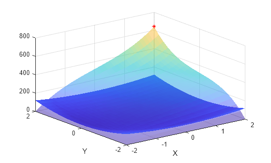
Perform nested integrations in the x and y directions. Plot the results to visualize the cumulative integral value in both directions.

Create a grid of values for the domain.

x = -2:0.1:2;
y = -2:0.2:2;
[X,Y] = meshgrid(x,y);

Calculate the function f(x,y)=10x2+20y2 on the grid.

F = 10*X.^2 + 20*Y.^2;

cumtrapz integrates numeric data rather than functional expressions, so in general the underlying function does not need to be known to use cumtrapz on a matrix of data. In cases where the functional expression is known, you can instead use integral, integral2, or integral3.

Use cumtrapz to approximate the double integral

I(a,b)=-2b-2a(10x2+20y2)dxdy.

To perform this double integration, use nested function calls to cumtrapz. The inner call first integrates the rows of data, then the outer call integrates the columns.

I = cumtrapz(y,cumtrapz(x,F,2));

Plot the surface representing the original function as well as the surface representing the cumulative integration. Each point on the surface of the cumulative integration gives an intermediate value of the double integral. The last value in I gives the overall approximation of the double integral, I(end) = 642.4. Mark this point in the plot with a red star.

surf(X,Y,F,'EdgeColor','none')
xlabel('X')
ylabel('Y')
hold on
surf(X,Y,I,'FaceAlpha',0.5,'EdgeColor','none')
plot3(X(end),Y(end),I(end),'r*')
hold off

Input Arguments

collapse all

Numeric data, specified as a vector, matrix, or multidimensional array. By default, cumtrapz integrates along the first dimension of Y whose size does not equal 1.

Data Types: single | double
Complex Number Support: Yes

Point spacing, specified as 1 (default), a uniform scalar spacing, or a vector of coordinates.

  • If X is a scalar, then it specifies a uniform spacing between the data points and cumtrapz(X,Y) is equivalent to X*cumtrapz(Y).

  • If X is a vector, then it specifies x-coordinates for the data points and length(X) must be the same as the size of the integration dimension in Y.

Data Types: single | double

Dimension to operate along, specified as a positive integer scalar. If you do not specify the dimension, then the default is the first array dimension of size greater than 1.

Consider a two-dimensional input array, Y:

  • cumtrapz(Y,1) works on successive elements in the columns of Y.

    cumtrapz(Y,1) column-wise computation

  • cumtrapz(Y,2) works on successive elements in the rows of Y.

    cumtrapz(Y,2) row-wise computation

If dim is greater than ndims(Y), then cumtrapz returns an array of zeros of the same size as Y.

Tips

  • Use trapz and cumtrapz to perform numerical integrations on discrete data sets. Use integral, integral2, or integral3 instead if a functional expression for the data is available.

  • trapz reduces the size of the dimension it operates on to 1, and returns only the final integration value. cumtrapz also returns the intermediate integration values, preserving the size of the dimension it operates on.
Extended Capabilities

C/C++ Code Generation
Generate C and C++ code using MATLAB® Coder™.

Version History

Introduced before R2006a