equilibrate
Matrix scaling for improved conditioning
Description
[
returns the outputs P,R,C] = equilibrate(A,outputForm)P, R, and C in
the form specified by outputForm. For example, you can specify
outputForm as "vector" to return the outputs as
column vectors.
Examples
Equilibrate a matrix with a large condition number to improve the efficiency and stability of a linear system solution with the iterative solver gmres.
Load the west0479 matrix, which is a real-valued 479-by-479 sparse matrix. Use condest to calculate the estimated condition number of the matrix.
load west0479
A = west0479;
c1 = condest(A)
c1 = 1.4244e+12
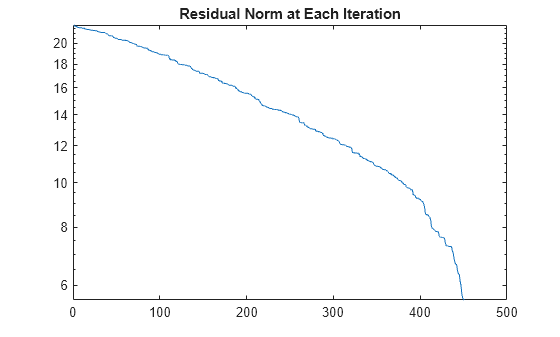
Try to solve the linear system using gmres with 450 iterations and a tolerance of 1e-11. Specify five outputs so that gmres returns the residual norms of the solution at each iteration (using ~ to suppress unneeded outputs). Plot the residual norms in a semilog plot. The plot shows that gmres is not able to achieve a reasonable residual norm, and so the calculated solution for is not reliable.
b = ones(size(A,1),1);
tol = 1e-11;
maxit = 450;
[x,flx,~,~,rvx] = gmres(A,b,[],tol,maxit);
semilogy(rvx)
title('Residual Norm at Each Iteration')
Use equilibrate to permute and rescale A. Create a new matrix B = R*P*A*C, which has a better condition number and diagonal entries of only 1 and -1.
[P,R,C] = equilibrate(A);
B = R*P*A*C;
c2 = condest(B)
c2 =
5.1036e+04
Using the outputs returned by equilibrate, you can reformulate the problem into , where and . In this form you can recover the solution to the original system with . The recovered solution, however, might not have the desired residual error for the original system. See Rescaling to Solve a Linear System for details.
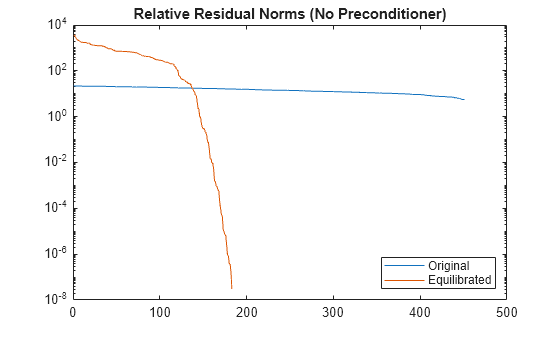
Use gmres to solve for , and then replot the residual norms at each iteration. The plot shows that equilibrating the matrix improves the stability of the problem, with gmres converging to the desired tolerance of 1e-11 in fewer than 200 iterations.
d = R*P*b;
[y,fly,~,~,rvy] = gmres(B,d,[],tol,maxit);
hold on
semilogy(rvy)
legend('Original', 'Equilibrated', 'Location', 'southeast')
title('Relative Residual Norms (No Preconditioner)')
hold off

Improve Solution with Preconditioner
After you obtain the matrix B, you can improve the stability of the problem even further by calculating a preconditioner for use with gmres. The numerical properties of B are better than those of the original matrix A, so you should use the equilibrated matrix to calculate the preconditioner.
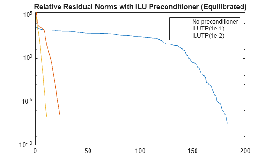
Calculate two different preconditioners with ilu, and use these as inputs to gmres to solve the problem again. Plot the residual norms at each iteration on the same plot as the equilibrated norms for comparison. The plot shows that calculating preconditioners with the equilibrated matrix greatly increases the stability of the problem, with gmres achieving the desired tolerance in fewer than 30 iterations.
semilogy(rvy)
hold on

[L1,U1] = ilu(B,struct('type','ilutp','droptol',1e-1,'thresh',0));
[yp1,flyp1,~,~,rvyp1] = gmres(B,d,[],tol,maxit,L1,U1);
semilogy(rvyp1)

[L2,U2] = ilu(B,struct('type','ilutp','droptol',1e-2,'thresh',0));
[yp2,flyp2,~,~,rvyp2] = gmres(B,d,[],tol,maxit,L2,U2);
semilogy(rvyp2)

legend('No preconditioner', 'ILUTP(1e-1)', 'ILUTP(1e-2)')
title('Relative Residual Norms with ILU Preconditioner (Equilibrated)')
hold off

Create a 6-by-6 magic square matrix, and then use equilibrate to factor the matrix. By default, equilibrate returns the permutation and scaling factors as matrices.
A = magic(6)
A = 6×6

    35     1     6    26    19    24
     3    32     7    21    23    25
    31     9     2    22    27    20
     8    28    33    17    10    15
    30     5    34    12    14    16
     4    36    29    13    18    11
[P,R,C] = equilibrate(A)
P = 6×6

     0     0     0     0     1     0
     0     0     0     0     0     1
     0     0     0     1     0     0
     1     0     0     0     0     0
     0     0     1     0     0     0
     0     1     0     0     0     0
R = 6×6

    0.1852         0         0         0         0         0
         0    0.1749         0         0         0         0
         0         0    0.1909         0         0         0
         0         0         0    0.1588         0         0
         0         0         0         0    0.1793         0
         0         0         0         0         0    0.1966
C = 6×6

    0.1799         0         0         0         0         0
         0    0.1588         0         0         0         0
         0         0    0.1588         0         0         0
         0         0         0    0.2422         0         0
         0         0         0         0    0.2066         0
         0         0         0         0         0    0.2035
Construct the equilibrated matrix Bmatrix using the matrix factors P, R, and C.
Bmatrix = R*P*A*C
Bmatrix = 6×6

    1.0000    0.1471    1.0000    0.5385    0.5358    0.6031
    0.1259    1.0000    0.8056    0.5509    0.6506    0.3916
    0.2747    0.8485    1.0000    0.7859    0.3943    0.5825
    1.0000    0.0252    0.1513    1.0000    0.6233    0.7754
    1.0000    0.2562    0.0569    0.9553    1.0000    0.7295
    0.1061    0.9988    0.2185    1.0000    0.9341    1.0000
Now, specify the "vector" option to return the outputs as vectors. With large input matrices, returning the outputs as vectors can save memory and improve efficiency.
[p,r,c] = equilibrate(A,"vector")p = 6×1
5
6
4
1
3
2
r = 6×1

    0.1852
    0.1749
    0.1909
    0.1588
    0.1793
    0.1966
c = 6×1

    0.1799
    0.1588
    0.1588
    0.2422
    0.2066
    0.2035
Construct the equilibrated matrix Bvector using the vector outputs p, r, and c.
Bvector = r.*A(p,:).*c'
Bvector = 6×6

    1.0000    0.1471    1.0000    0.5385    0.5358    0.6031
    0.1259    1.0000    0.8056    0.5509    0.6506    0.3916
    0.2747    0.8485    1.0000    0.7859    0.3943    0.5825
    1.0000    0.0252    0.1513    1.0000    0.6233    0.7754
    1.0000    0.2562    0.0569    0.9553    1.0000    0.7295
    0.1061    0.9988    0.2185    1.0000    0.9341    1.0000
Compare Bvector and Bmatrix. The result indicates they are equal.
norm(Bmatrix - Bvector)
ans =
0
Input Arguments
Input matrix, specified as a square matrix. A can be dense or
sparse, but must be structurally nonsingular, as determined by sprank.
When A is sparse, the outputs P,
R, and C are also sparse.
Data Types: single | double
Complex Number Support: Yes
Output format, specified as "vector" or
"matrix". This option allows you to specify whether the outputs
P, R, and C are
returned as column vectors or as matrices:
"matrix"—P,R, andCare matrices such thatB = R*P*A*C."vector"—P,R, andCare column vectors such thatB = R.*A(P,:).*C'.
Example: [P,R,C] = equilibrate(A,"vector") returns
P, R, and C as
vectors.
Output Arguments
Permutation information, returned as a matrix or vector. P*A (or
A(P,:) with the "vector" option) is the
permutation of A that maximizes the absolute value of the product of
its diagonal elements.
Row scaling, returned as a diagonal matrix or vector. The nonzero entries in
R and C are real and positive.
Column scaling, returned as a diagonal matrix or vector. The nonzero entries in
R and C are real and positive.
More About
For linear system solutions x = A\b, the condition
number of A is important for accuracy and efficiency of the calculation.
equilibrate can improve the condition number of A
by rescaling the basis vectors. This effectively forms a new coordinate system that both
b and x can be expressed in.
equilibrate is most useful when the scales of the
b and x vectors in the original system x =
A\b are irrelevant. However, if the scales of b and
x
are relevant, then using equilibrate to rescale
A only for the linear system solve is not recommended. The obtained
solution does not generally yield a small residual for the original system, even if
expressed using the original basis vectors.
References
[1] Duff, I. S., and J. Koster. “On Algorithms For Permuting Large Entries to the Diagonal of a Sparse Matrix.” SIAM Journal on Matrix Analysis and Applications 22, no. 4 (January 2001): 973–96.
Extended Capabilities
The equilibrate function fully supports
thread-based environments. For more information, see Run MATLAB Functions in Thread-Based Environment.
Version History
Introduced in R2019aSpecify outputForm as "vector" or
"matrix" to control whether equilibrate returns
the output arguments as vectors or matrices. For large factorizations, returning the outputs
as vectors can save memory and improve efficiency.
MATLAB Command
You clicked a link that corresponds to this MATLAB command:
Run the command by entering it in the MATLAB Command Window. Web browsers do not support MATLAB commands.
Select a Web Site
Choose a web site to get translated content where available and see local events and offers. Based on your location, we recommend that you select: .
You can also select a web site from the following list
How to Get Best Site Performance
Select the China site (in Chinese or English) for best site performance. Other MathWorks country sites are not optimized for visits from your location.
Americas
- América Latina (Español)
- Canada (English)
- United States (English)
Europe
- Belgium (English)
- Denmark (English)
- Deutschland (Deutsch)
- España (Español)
- Finland (English)
- France (Français)
- Ireland (English)
- Italia (Italiano)
- Luxembourg (English)
- Netherlands (English)
- Norway (English)
- Österreich (Deutsch)
- Portugal (English)
- Sweden (English)
- Switzerland
- United Kingdom (English)