Tune Weights
A model predictive controller design usually requires some tuning of the cost function weights. This topic provides tuning tips. See QP Optimization Problem for Linear MPC for details on the cost function equations.
Initial Tuning
Before tuning the cost function weights, specify scale factors for each plant input and output variable. Hold these scale factors constant as you tune the controller. See Specify Scale Factors for more information.
During tuning, you can use the
sensitivityandreviewcommands to obtain diagnostic feedback. Thesensitivitycommand is intended to help with cost function weight selection.Change a weight by setting the appropriate controller property, as follows:
To change this weight Set this controller property Array size OV reference tracking (wy) Weights.OVp-by-ny MV reference tracking (wu) Weights.MVp-by-nu MV increment suppression (wΔu) Weights.MVRatep-by-nu
Here, MV is a plant manipulated variable, and nu is the number of MVs. OV is a plant output variable, and ny is the number of OVs. Finally,p is the number of steps in the prediction horizon.
If a weight array contains n < p rows, the controller duplicates the last row to obtain a full array of p rows. The default (n = 1) minimizes the number of parameters to be tuned, and is therefore recommended. See Setting Time-Varying Weights and Constraints with MPC Designer for an alternative.
Tips for Setting OV Weights
Considering the ny OVs, suppose that nyc must be held at or near a reference value (setpoint). If the ith OV is not in this group, set
Weights.OV(:,i)= 0.If nu ≥ nyc, it is usually possible to achieve zero OV tracking error at steady state, if at least nyc MVs are not constrained. The default
Weights.OV = ones(1,ny)is a good starting point in this case.If nu > nyc, however, you have excess degrees of freedom. Unless you take preventive measures, therefore, the MVs might drift even when the OVs are near their reference values.
The most common preventive measure is to define reference values (targets) for the number of excess MVs you have, nu – nyc. Such targets can represent economically or technically desirable steady-state values.
An alternative measure is to set w∆u > 0 for at least nu – nyc MVs to discourage the controller from changing them.
If nu < nyc, you do not have enough degrees of freedom to simultaneously keep all OVs at a setpoint. In this case, consider prioritizing reference tracking. To do so, set
Weights.OV(:,i) >
                0
to specify the priority for the ith OV. Rough guidelines for this are as follows:0.05 — Low priority: Large tracking error acceptable
0.2 — Below-average priority
1 — Average priority – the default. Use this value if nyc = 1.
5 — Above average priority
20 — High priority: Small tracking error desired
Tips for Setting MV Weights
By default, Weights.MV = zeros(1,nu). If some MVs have targets, the
corresponding MV reference tracking weights must be nonzero. Otherwise, the targets are
ignored. If the number of MV targets is less than
(nu –
nyc), try using the same weight for each. A
suggested value is 0.2, the same as below-average OV tracking. This value allows the MVs
to move away from their targets temporarily to improve OV tracking.
Otherwise, the MV and OV reference tracking goals are likely to conflict. Prioritize
by setting the Weights.MV(:,i) values in a manner similar to that
suggested for Weights.OV (see above). Typical practice sets the average
MV tracking priority lower than the average OV tracking priority (e.g., 0.2 <
1).
If the ith MV does not have a target, set
Weights.MV(:,i) = 0 (the default).
Tips for Setting MV Rate Weights
By default,
Weights.MVRate = 0.1*ones(1,nu). The reasons for this default include:If the plant is open-loop stable, large increments are unnecessary and probably undesirable. For example, when model predictions are imperfect, as is always the case in practice, more conservative increments usually provide more robust controller performance, but poorer reference tracking.
These values force the QP Hessian matrix to be positive-definite, such that the QP has a unique solution if no constraints are active.
To encourage the controller to use even smaller increments for the ith MV, increase the
Weights.MVRate(:,i)value.If the plant is open-loop unstable, you might need to decrease the average
Weight.MVRatevalue to allow sufficiently rapid response to upsets.
Tips for Setting ECR Weights
See Constraint Softening for tips regarding the Weights.ECR
property.
Testing and Refinement
To focus on tuning individual cost function weights, perform closed-loop simulation tests under the following conditions:
No constraints.
No prediction error. The controller prediction model should be identical to the plant model. Both the MPC Designer app and the
simfunction provide the option to simulate under these conditions.
Use changes in the reference and measured disturbance signals (if any) to force a dynamic response. Based on the results of each test, consider changing the magnitudes of selected weights.
One suggested approach is to use constant Weights.OV(:,i) = 1
indicating “average OV tracking priority,” and adjust all other weights to be
relative to this value. Use the sensitivity command for guidance. Use the
review command to check for typical tuning issues, such as lack of closed-loop
stability.
See Adjust Disturbance and Noise Models for tests focusing on the disturbance rejection ability of the controller.
Robustness
Once you have weights that work well under the above conditions, check for sensitivity to prediction error. There are several ways to do so:
If you have a nonlinear plant model of your system, such as a Simulink® model, simulate the closed-loop performance at operating points other than that for which the LTI prediction model applies.
Alternatively, run closed-loop simulations in which the LTI model representing the plant differs (such as in structure or parameter values) from that used at the MPC prediction model. Both the MPC Designer app and the
simfunction provide the option to simulate under these conditions. For an example, see Test MPC Controller Robustness Using MPC Designer.
If controller performance seems to degrade significantly in comparison to tests with no prediction error, for an open-loop stable plant, consider making the controller less aggressive.
In MPC Designer, on the Tuning tab, you can do so using the Closed-Loop Performance slider.
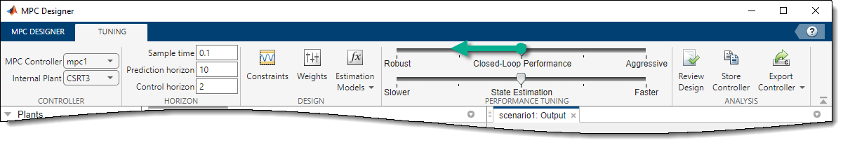
Moving toward more robust control decreases both OV and MV weights and increases MV Rate weights, which leads to relaxed control of outputs and more conservative control moves.
At the command line, you can make the following changes to decrease controller aggressiveness:
Increase all
Weight.MVRatevalues by a multiplicative factor of order 2.Decrease all
Weight.OVandWeight.MVvalues by dividing by the same factor.
After adjusting the weights, reevaluate performance both with and without prediction error.
If both are now acceptable, stop tuning the weights.
If there is improvement but still too much degradation with model error, increase the controller robustness further.
If the change does not noticeably improve performance, restore the original weights and focus on state estimator tuning (see Adjust Disturbance and Noise Models).
Finally, if tuning changes do not provide adequate robustness, consider one of the following options:
See Also
Functions
size|review|sensitivity